BERT, explained · Part 6 of 6 · Covers §6 and later work

After BERT: Impact, Limits and Summary

The paper's conclusion, what came next (RoBERTa, ALBERT, DistilBERT, ELECTRA, Sentence-BERT and more), BERT's real limits measured on real models, how BERT-style models are used today, and the whole paper summarised on one page.

BERT: Pre-training of Deep Bidirectional Transformers for Language Understanding. Jacob Devlin, Ming-Wei Chang, Kenton Lee, Kristina Toutanova. NAACL 2019, 2018. arXiv:1810.04805

This is the last part. We have read every section of the paper: the idea (Part 1), the model and its input (Part 2), pre-training (Part 3), fine-tuning and results (Part 4) and the ablations (Part 5). Only the short conclusion is left.

After that, this part steps outside the paper. It answers three questions: what did other researchers change after BERT, what can BERT not do, and how are BERT-style models used today. Every claim about later work comes from that work's own paper or post, linked at the end. The measurements come from a script you can run.

The conclusion#

Three phrases need unpacking.

"Even low-resource tasks benefit from deep unidirectional architectures." This sentence is about the work before BERT, mainly OpenAI GPT. GPT showed that a deep, left-to-right model, pre-trained on plain text, makes even small tasks work well, because the task no longer has to teach the model language from scratch.

"Our major contribution is further generalizing these findings to deep bidirectional architectures." BERT keeps that recipe and changes one thing: the direction. The masked language model (Part 3) is what made it possible to pre-train a model that looks both ways in every layer. The ablations in Part 5 showed that this one change is where most of the gain comes from.

"The same pre-trained model." One download, many tasks. This is the practical part of the conclusion, and it is why BERT spread so fast.

What happened next#

The paper's code and weights were public from the start, so other researchers could build on it right away. The years 2019 and 2020 brought a wave of follow-up models.

Two events show how quickly BERT mattered outside research:

• In June 2019 the paper won the Best Long Paper award at NAACL 2019, the conference where it was published.
• On 25 October 2019, Google wrote that BERT "will help Search better understand one in 10 searches in the U.S. in English". The same post says Google also applied a BERT model to improve featured snippets "in the two dozen countries where this feature is available".

The follow-up models changed BERT in four different directions.

1. Train the same model better: RoBERTa and SpanBERT#

RoBERTa (Liu et al., July 2019) is a careful replication of BERT. Its abstract says plainly: "We find that BERT was significantly undertrained." With the same architecture, they changed only the training: "(1) training the model longer, with bigger batches, over more data; (2) removing the next sentence prediction objective; (3) training on longer sequences; and (4) dynamically changing the masking pattern applied to the training data." They trained on over 160GB of text instead of BERT's 16GB (Wikipedia plus books, in their measurement).

The NSP result is interesting, because it seems to contradict BERT's own Table 5 (Part 5), where removing NSP hurt. RoBERTa found that "removing the NSP loss matches or slightly improves downstream task performance". They offer a possible reason: "the original BERT implementation may only have removed the loss term while still retaining the SEGMENT-PAIR input format". In other words, BERT's "No NSP" model still trained on pairs of shorter text pieces; RoBERTa's trained on long, full blocks of text. Both results can be true, because they removed NSP in different ways.

SpanBERT (Joshi et al., July 2019) masks "contiguous random spans, rather than random tokens", and gains most on "span selection tasks such as question answering and coreference resolution". Its abstract reports 94.6 F1 on SQuAD 1.1 and 88.7 on SQuAD 2.0, "with the same training data and model size as BERT-large".

2. Make it smaller: ALBERT and DistilBERT#

ALBERT (Lan et al., September 2019) uses "two parameter-reduction techniques":

• factorized embedding parameterization: the big vocabulary table is split into two small matrices, so its size no longer grows with the hidden size;
• cross-layer parameter sharing: all layers share the same weights, so the size no longer grows with the depth.

ALBERT also replaces NSP with sentence-order prediction (SOP), a task about "inter-sentence coherence": are these two consecutive pieces in the right order or swapped? The paper describes it as designed to address "the ineffectiveness" of NSP. Their example of the size saving: "ALBERT-large has about 18x fewer parameters compared to BERT-large, 18M versus 334M".

DistilBERT (Sanh et al., October 2019) uses distillation during pre-training. Its abstract: "it is possible to reduce the size of a BERT model by 40%, while retaining 97% of its language understanding capabilities and being 60% faster."

The distillation loss, for one masked position, compares the student's probabilities $s$ with the teacher's $t$ over the vocabulary:

where $y$ is the true word and the sum runs over every word $w$ of the vocabulary. The hard loss only rewards the right answer; the soft loss also rewards giving the teacher's runner-ups some probability. (DistilBERT combines this soft loss with the masked-LM loss and a cosine loss on the hidden vectors; here we show only the idea.) Measured on "i went to the [MASK] to deposit my paycheck." (bert_part6_math.py):

encoder parameters: teacher 108,891,648 (12 layers), student 66,362,880 (6 layers), ratio 0.609
teacher top 5: bank 0.901, office 0.009, store 0.008, teller 0.008, atm 0.006
student top 5: bank 0.365, store 0.035, mall 0.025, hotel 0.022, supermarket 0.020
hard-label loss  -log s(bank)               = 1.009
soft-target loss -sum_w t(w) log s(w)       = 1.467   (teacher entropy, the smallest possible value: 0.774)

The student has 0.609 of the teacher's encoder weights, the "40% smaller" of the abstract. The soft loss can never go below the teacher's own entropy (0.774 here), reached only when the student copies the teacher exactly.

3. Fix the masked language model: XLNet, ELECTRA and DeBERTa#

The masked LM has two weak spots, and two papers named them directly. We measure both later in this part.

XLNet (Yang et al., June 2019) says that "relying on corrupting the input with masks, BERT neglects dependency between the masked positions and suffers from a pretrain-finetune discrepancy". XLNet keeps bidirectional context but predicts words in many different random orders instead of using [MASK].

ELECTRA (Clark et al., March 2020) points at a different cost: BERT only learns from the masked tokens. ELECTRA replaces some tokens with "plausible alternatives sampled from a small generator network", then trains the main model to say, for every token, whether it was replaced. This is "more efficient than MLM because the task is defined over all input tokens rather than just the small subset that was masked out". Its abstract gives an example: "we train a model on one GPU for 4 days that outperforms GPT (trained using 30x more compute) on the GLUE natural language understanding benchmark".

DeBERTa (He et al., June 2020) changes attention itself: "each word is represented using two vectors that encode its content and position", instead of one vector that adds them together as BERT does (Part 2).

4. Use it differently: Sentence-BERT, and a modern BERT#

Sentence-BERT (Reimers and Gurevych, August 2019) fixed a problem the paper itself warns about in footnote 6: BERT's [CLS] vector is not a good sentence vector without fine-tuning. Sentence-BERT says that averaging BERT's outputs or using the [CLS] output "yields rather bad sentence embeddings, often worse than averaging GloVe embeddings". It fine-tunes BERT so that sentences with similar meanings get similar vectors. We test this ourselves below.

ModernBERT (Warner et al., December 2024) shows the idea is still alive. It calls encoder-only models like BERT "the workhorse of numerous production pipelines", and brings modern training to them: "Trained on 2 trillion tokens with a native 8192 sequence length". Compare that with BERT's 512 tokens.

BERT's limits, measured#

Every model has limits. Here are BERT's main ones. Where the paper itself mentions a limit, its lines are shown; where a limit can be measured, I measured it with bert_part6.py on the public bert-base-uncased model.

Limit 1: at most 512 tokens#

Recall from Part 2 that BERT adds a position embedding to every token, looked up in a table with one row per position. The code reads the size of that table and then tries a long input:

bert = AutoModel.from_pretrained("bert-base-uncased")
print(bert.embeddings.position_embeddings.weight.shape)     # rows = positions it knows

long_text = " ".join(["BERT reads the whole input at once, so every token can look at every other token."] * 40)
print(len(tok(long_text).input_ids))                                   # all tokens
print(len(tok(long_text, truncation=True, max_length=512).input_ids))  # what is kept
bert(**tok(long_text, return_tensors="pt"))                            # try all of them

1. The 512-token limit
   position embedding table: 512 rows x 768 numbers
   a long text has 722 tokens; with truncation it keeps 512; the rest is thrown away
   feeding all 722 tokens: RuntimeError: The size of tensor a (722) must match the size of tensor b (512) at non-singleton dimension 1

The table has exactly 512 rows. A 722-token text either crashes the model or loses its last 210 tokens. A few long paragraphs are already too much, so long documents have to be cut into pieces. This is the limit ModernBERT's 8192-token context attacks.

The usual workaround, used by the released SQuAD code (Part 4), is to read a long text in overlapping windows. With window size $w$ content tokens (510, leaving room for [CLS] and [SEP]) and step $s$ between window starts, a text of $N$ tokens needs

where $\lceil \cdot \rceil$ rounds up. For $N = 720$, $w = 510$, $s = 382$: $k = 1 + \lceil 210 / 382 \rceil = 2$. Windows also keep the attention cost linear in $N$: each window costs $512^2$ per head and layer, so $k \times 512^2$ in total, against $(N + 2)^2$ for one long input (if the model could take it):

N =    720: windows =   2; one long input (N+2)^2 =     521,284; windows k*512^2 =     524,288; ratio 0.99
N =   2000: windows =   5; one long input (N+2)^2 =   4,008,004; windows k*512^2 =   1,310,720; ratio 3.06
N =  10000: windows =  26; one long input (N+2)^2 = 100,040,004; windows k*512^2 =   6,815,744; ratio 14.68

The price: a token in window 1 never sees a token in window 2. Facts that are far apart in a long document cannot be combined. That is the real cost of the 512 wall, and why later models raised it.

Limit 2: [MASK] never appears after pre-training#

During pre-training, BERT sees [MASK] in about 12% of positions (80% of the 15% chosen). In real use it never sees [MASK] at all. Part 3 explained the 80% / 10% / 10% trick that reduces the gap, and Part 5 (Table 8) measured how much it matters. XLNet named this the "pretrain-finetune discrepancy".

Limit 3: only 15% of tokens teach the model#

Part 5 (Appendix C.1) showed that BERT does learn a little more slowly because of this, but still wins. ELECTRA turned this observation into a new pre-training task.

Limit 4: two blanks are filled separately#

When BERT fills several [MASK]s at once, it predicts each one on its own. It does not know what it put in the other blank. I masked both words of a two-word city name:

3. Two [MASK]s at once: each one is predicted on its own
   i flew from [MASK] [MASK] to london last week.
     mask 1: new 0.042, the 0.037, chicago 0.037, la 0.028, portland 0.019
     mask 2: town 0.068, york 0.044, beach 0.025, city 0.021, ##town 0.017
   i flew from new [MASK] to london last week.  -> york 0.979, orleans 0.012, jersey 0.003
   i flew from los [MASK] to london last week.  -> angeles 1.000, vegas 0.000, ' 0.000
   i flew from hong [MASK] to london last week. -> kong 0.999, ##kong 0.001, china 0.000

Taking the top guess for each blank separately gives "new town". But once the first word is filled in, the second becomes almost certain: "york" (0.979) after "new", "angeles" after "los", "kong" after "hong". The two blanks depend on each other, and BERT's masked LM cannot use that when both are hidden. This is what XLNet meant by "neglects dependency between the masked positions".

In equations, the masked LM scores the two blanks $a$ and $b$ as if they were independent, while the true probability follows the chain rule of Part 1:

"new town":  p(a) = 0.0424, p(b) = 0.0678, p(b | a) = 0.0000
   independent p(a) p(b) = 0.002876;  chain rule p(a) p(b | a) = 0.000000
"new york":  p(a) = 0.0424, p(b) = 0.0440, p(b | a) = 0.9794
   independent p(a) p(b) = 0.001868;  chain rule p(a) p(b | a) = 0.041548
best pair by the independent score (over 29 candidate pairs): "new town" 0.002876
best pair by the chain rule:                                  "new york" 0.041548

Limit 5: no ready-made sentence vector#

The formula, $\cos(a, b) = a \cdot b \,/\, (\lVert a \rVert \lVert b \rVert)$, on one real pair of [CLS] vectors:

a = C("A man is playing a guitar."), b = C("A person is making music."), each with 768 numbers
a . b = 199.086;  |a| = 15.498;  |b| = 15.086
cos = a . b / (|a| |b|) = 199.086 / (15.498 x 15.086) = 0.851   (torch: 0.851)
toy check in 2-D: a = (3, 4), b = (4, 3): a . b = 24, |a| = |b| = 5, cos = 24 / 25 = 0.96

I compared six sentence pairs, three related and three unrelated, with three kinds of vector:

• raw BERT [CLS]: the vector C of bert-base-uncased, as the footnote warns against;
• raw BERT, mean of tokens: the average of all of BERT's output vectors;
• all-MiniLM-L6-v2: a public model from the Sentence-BERT authors' library. Its config says model_type=bert, so it has BERT's architecture, but it is a small distilled model (6 layers, 384 numbers per token, 22.7M parameters, from the script's output), fine-tuned on over 1 billion sentence pairs (its model card) to make similar sentences close.

   pair (R = related, U = unrelated)                                   raw [CLS]  raw mean  MiniLM
   R A man is playing a guitar.   | A person is making music.              0.851     0.746   0.590
   R How do I reset my password?  | I forgot my login details.             0.929     0.672   0.541
   R The weather is lovely today. | It is sunny and warm outside.          0.951     0.857   0.705
   U A man is playing a guitar.   | The stock market fell sharply.         0.776     0.584  -0.064
   U How do I reset my password?  | Penguins live in Antarctica.           0.795     0.517  -0.035
   U The weather is lovely today. | He parked the truck in the garage.     0.873     0.598   0.013
   average related / unrelated:  raw [CLS] 0.910 / 0.815,  raw mean 0.758 / 0.566,  MiniLM 0.612 / -0.029

What the numbers say:

• Raw [CLS] says everything is similar. Even "the weather is lovely" and "he parked the truck in the garage" get 0.873, higher than the related guitar pair (0.851). You cannot pick a threshold that separates the two groups. The footnote is right.
• Averaging BERT's outputs is better but not clean: related pairs average 0.758 and unrelated 0.566, but the gap is small.
• A model fine-tuned for similarity separates them clearly: unrelated pairs score between -0.064 and 0.013, related pairs between 0.541 and 0.705.

This is only six pairs, so treat it as an illustration, not a benchmark. Sentence-BERT's paper measures the same effect on standard similarity datasets.

Limit 6: it does not write text#

BERT is an encoder. It reads a whole input and gives back one vector per token; it has no natural way to write a long answer one word at a time. As footnote 4 of the paper puts it (Part 2), the left-context-only Transformer is called a "Transformer decoder" "since it can be used for text generation". Chatbots are built on decoders, in the line of GPT, not on BERT.

Limit 7: pre-training is expensive#

The good news is the paper's own: fine-tuning is cheap. Section 3.2 says every result in the paper "can be replicated in at most 1 hour on a single Cloud TPU, or a few hours on a GPU, starting from the exact same pre-trained model" (Part 4).

How big was the pre-training budget, in tokens? From the numbers in Appendix A.2:

tokens per batch = 256 x 512 = 131,072  (the paper rounds to 128,000)
tokens seen      = 1,000,000 steps x 131,072 = 131,072,000,000  (an upper bound: 90% of steps use length 128)
with 90% of steps at length 128 and 10% at 512: 1,000,000 x 256 x (0.9 x 128 + 0.1 x 512) = 42,598,400,000
predicted tokens (15%) of that: 6,389,760,000
chip-days: BERT-base 16 chips x 4 days = 64; BERT-large 64 chips x 4 days = 256

One subtlety: the paper's "approximately 40 epochs over the 3.3 billion word corpus" matches the upper bound (131 billion tokens ÷ 3.3 billion words ≈ 40). If the batch stayed at 256 sequences during the length-128 phase, the model saw about 42.6 billion tokens, roughly 13 passes. The paper does not say whether the batch size changed between the two phases, so the exact number of epochs cannot be recovered from the text.

How BERT-style models are used today#

Large chatbots get the headlines, but small encoders like BERT do a lot of quiet work, because they are fast and cheap to run on every piece of text. ModernBERT's authors call them "the workhorse of numerous production pipelines". Typical jobs:

• Classification: spam or not, which team should handle this support ticket, is this review positive. This is the GLUE recipe from Part 4: [CLS] vector, one layer, fine-tune.
• Finding names and things (NER): people, places, products, drug names in text. This is the token-level recipe from Part 4.
• Search and retrieval: sentence-embedding models in the Sentence-BERT line turn every document into a vector once, then compare vectors at search time. This is how many "chat with your documents" systems find the right passages.
• Reranking: a cross-encoder reads the question and one candidate passage together, exactly like BERT's sentence pairs, and scores how well they match. Sentence-BERT describes BERT itself as a cross-encoder: "Two sentences are passed to the transformer network". It is accurate but slow, so it is used to re-order a short list found by the faster vector search.

Here is the NER use case with a real public checkpoint, dslim/bert-base-NER. Its model card says it is bert-base-cased fine-tuned on the CoNLL-2003 dataset (the same NER task as the paper's Section 5.3), with four entity types: person (PER), location (LOC), organisation (ORG) and miscellaneous (MISC).

from transformers import pipeline
ner = pipeline("ner", model="dslim/bert-base-NER", aggregation_strategy="simple")
ner("Ada Lovelace was born in London and worked with Charles Babbage on the Analytical Engine.")

4. Named entities with dslim/bert-base-NER (BERT-base-cased fine-tuned on CoNLL-2003)
   Ada Lovelace was born in London and worked with Charles Babbage on the Analytical Engine.
     Ada Lovelace           PER   0.999
     London                 LOC   0.999
     Charles Babbage        PER   0.932
     Analy                  ORG   0.723
     Engine                 ORG   0.781
   token by token, for "Analytical Engine":
     Ana                    B-ORG  0.901
     ##ly                   I-ORG  0.544
     Engine                 I-ORG  0.781

The people and the place are found with high confidence. "Analytical Engine" (a machine, not really an organisation) shows a real rough edge: WordPiece split "Analytical" into Ana, ##ly and ##tical, the last piece got no entity label, and the result came out broken into "Analy" and "Engine". The model card warns about exactly this: the model "occassionally tags subword tokens as entities". This is why Section 5.3 of the paper labels only the first sub-token of each word (Part 5).

The whole paper on one page#

Here is the paper, part by part, with its key numbers. Every number is from the paper, with its location.

Part 1: The Big Idea (Abstract, §1). Language models read in one direction, which is a real limit for tasks like question answering, where "it is crucial to incorporate context from both directions" (§1). BERT pre-trains a deep bidirectional Transformer by hiding words and predicting them. It set new state-of-the-art results on eleven tasks, including GLUE 80.5 (+7.7 points), MultiNLI 86.7% (+4.6), SQuAD v1.1 Test F1 93.2 (+1.5) and SQuAD v2.0 Test F1 83.1 (+5.1) (Abstract).

Part 2: Inside BERT (§2, §3). BERT is a Transformer encoder. BERT-base has L=12 layers, H=768, A=12 heads and 110M parameters; BERT-large has L=24, H=1024, A=16 and 340M (§3). The feed-forward size is 4H: 3072 and 4096 (footnote 3). Text is cut into WordPiece tokens from a 30,000-token vocabulary; every input starts with [CLS], sentences are separated by [SEP], and each token's input is the sum of a token, a segment and a position embedding (§3, Figure 2).

Part 3: Pre-training (§3.1, A.1, A.2). Masked LM: choose 15% of the WordPiece tokens; replace them with [MASK] 80% of the time, a random token 10% and leave them unchanged 10% (§3.1); random replacement is then only 1.5% of all tokens (A.1). Next sentence prediction: half the time sentence B really follows A (IsNext), half the time it is random (NotNext); the final model reaches 97%-98% on it (footnote 5). Data: BooksCorpus (800M words) and English Wikipedia (2,500M words) (§3.1). Training: batches of 256 sequences of 512 tokens ("128,000 tokens/batch") for 1,000,000 steps, "approximately 40 epochs over the 3.3 billion word corpus", Adam with learning rate 1e-4, 10,000 warm-up steps, dropout 0.1, GELU, 90% of the steps at length 128 (A.2).

Part 4: Fine-tuning and Results (§3.2, §4, A.3, A.5, B.1). For classification, the only new weights are W of size K×H, and the loss is $\log(\text{softmax}(CW^\top))$ (§4.1). On GLUE, BERT-base and BERT-large average 79.6 and 82.1, against 75.1 for OpenAI GPT (Table 1); on the official leaderboard BERT-large scores 80.5 against GPT's 72.8 (§4.1). For SQuAD, only a start vector S and an end vector E are new; a span from i to j scores $S \cdot T_i + E \cdot T_j$ with $j \ge i$ (§4.2). SQuAD v1.1 best Test F1 93.2 (ensemble with TriviaQA, Table 2); SQuAD v2.0 Test F1 83.1, +5.1 over the previous best (§4.3, Table 3); SWAG test accuracy 86.3, +27.1% over ESIM+ELMo and +8.3% over GPT (§4.4, Table 4). Good fine-tuning settings: batch size 16 or 32, learning rate 5e-5, 3e-5 or 2e-5, and 2, 3 or 4 epochs (A.3).

Part 5: Ablations (§5, A.4, C.1, C.2). Removing NSP hurts (MNLI 84.4 → 83.9, QNLI 88.4 → 84.9); training left-to-right hurts much more (MRPC 77.5, SQuAD F1 77.8 instead of 86.7 and 88.5) (Table 5). Bigger models are better on every task tried, from 3 layers to 24 (Table 6). Using BERT's frozen features (concatenating the last four layers) is "only 0.3 F1 behind fine-tuning the entire model" on named entity recognition (§5.3, Table 7). Training for 1M steps instead of 500k adds "almost 1.0%" on MNLI (C.1), and the 80/10/10 masking mix gives the best named entity recognition results, especially in the feature-based setting, while MNLI barely changes (Table 8).

This part (§6). The contribution is to generalise unsupervised pre-training "to deep bidirectional architectures" so "the same pre-trained model" can do many tasks (§6).

The key words, in one list#

Each term links to the part where it is first explained.

• Pre-training, fine-tuning, encoder, feature-based approach, language model, unidirectional, Cloze task: Part 1
• Transfer learning, L / H / A, parameters, WordPiece, [CLS] and [SEP], segment and position embeddings: Part 2
• Masked LM, the 80 / 10 / 10 rule, next sentence prediction, cross-entropy loss, perplexity, warm-up, GELU: Part 3
• GLUE, SQuAD, span, F1 and exact match, SWAG, dev and test sets: Part 4
• Ablation, feature extraction from layers, masking strategies: Part 5
• Dynamic masking, distillation, sentence embedding, cross-encoder: this part

Run it yourself

Every measurement in this part comes from code/papers/bert/bert_part6.py. It runs on a laptop CPU in about a minute and downloads bert-base-uncased, sentence-transformers/all-MiniLM-L6-v2 and dslim/bert-base-NER the first time.

bashCopy

pip install torch transformers
python bert_part6.py      # prints everything above, writes results/part6.json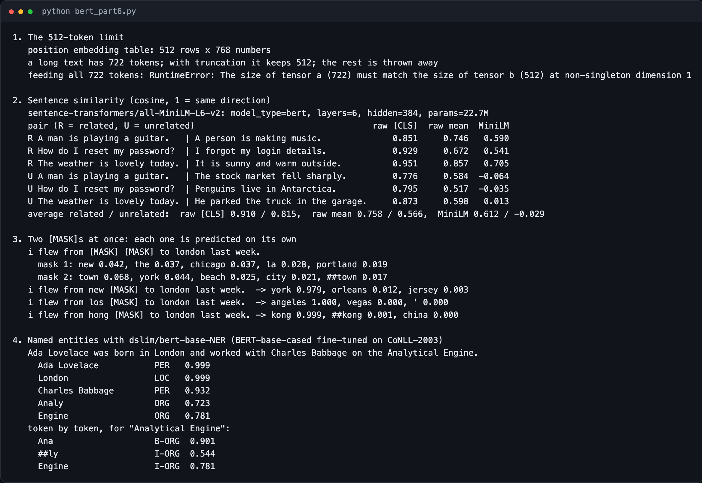

References#

The BERT paper

1. J. Devlin, M.-W. Chang, K. Lee, K. Toutanova. BERT: Pre-training of Deep Bidirectional Transformers for Language Understanding. NAACL 2019 (ACL Anthology). Best Long Paper at NAACL 2019.
2. Google Research. BERT code and pre-trained models.

Later work discussed in this part

3. Y. Liu et al. RoBERTa: A Robustly Optimized BERT Pretraining Approach. arXiv 2019.
4. M. Joshi, D. Chen, Y. Liu, D. S. Weld, L. Zettlemoyer, O. Levy. SpanBERT: Improving Pre-training by Representing and Predicting Spans. TACL 2020.
5. Z. Lan et al. ALBERT: A Lite BERT for Self-supervised Learning of Language Representations. ICLR 2020.
6. V. Sanh, L. Debut, J. Chaumond, T. Wolf. DistilBERT, a distilled version of BERT: smaller, faster, cheaper and lighter. NeurIPS EMC² workshop 2019.
7. Z. Yang, Z. Dai, Y. Yang, J. Carbonell, R. Salakhutdinov, Q. V. Le. XLNet: Generalized Autoregressive Pretraining for Language Understanding. NeurIPS 2019.
8. K. Clark, M.-T. Luong, Q. V. Le, C. D. Manning. ELECTRA: Pre-training Text Encoders as Discriminators Rather Than Generators. ICLR 2020.
9. P. He, X. Liu, J. Gao, W. Chen. DeBERTa: Decoding-enhanced BERT with Disentangled Attention. ICLR 2021.
10. N. Reimers, I. Gurevych. Sentence-BERT: Sentence Embeddings using Siamese BERT-Networks. EMNLP 2019.
11. B. Warner et al. Smarter, Better, Faster, Longer: A Modern Bidirectional Encoder for Fast, Memory Efficient, and Long Context Finetuning and Inference (ModernBERT). arXiv 2024.
12. G. Hinton, O. Vinyals, J. Dean. Distilling the Knowledge in a Neural Network. NeurIPS Deep Learning workshop 2014.

Other sources used in this part

13. P. Nayak. Understanding searches better than ever before. Google blog, 25 October 2019.
14. Public models used in the code: distilbert-base-uncased and sentence-transformers/all-MiniLM-L6-v2.
15. Code for this part: bert_part6.py and bert_part6_math.py.