BERT, explained · Part 3 of 6 · Covers §3.1, A.1, A.2

Pre-training: Masked LM and Next Sentence Prediction

Section 3.1 and Appendices A.1 and A.2 of the BERT paper, line by line: why a normal language model cannot look both ways, the masked language model and its 80/10/10 rule, next sentence prediction, the training data and the full training recipe. Every claim run on the real model or measured in code.

BERT: Pre-training of Deep Bidirectional Transformers for Language Understanding. Jacob Devlin, Ming-Wei Chang, Kenton Lee, Kristina Toutanova. NAACL 2019, 2018. arXiv:1810.04805

Part 2 built the model: a stack of Transformer layers that turns tokens into vectors. But a freshly built model knows nothing. Its millions of weights are random numbers.

This part is about how BERT learns language from plain text, before any real task. The paper uses two training games: fill in the blanks (the masked language model) and does this sentence come next? (next sentence prediction). We go through Section 3.1 paragraph by paragraph, then the two appendices that give the exact recipe, and we run every piece on the real model.

Not a normal language model#

Why not just look both ways?#

Here is the problem. Say we want every position to predict its own word from all the other words. In one layer, that is fine: we can simply forbid each position from looking at itself. But BERT has 12 layers, and information moves sideways at every layer.

So with two or more layers, every word can find its own answer by going through a neighbour. Training would then learn to copy, not to understand. That is what "trivially predict the target word in a multi-layered context" means.

A real experiment: watch a model cheat#

I trained three tiny Transformers on the same real text (WikiText-2, a public set of Wikipedia articles) and measured how well each predicts words. Each has 128 numbers per token and 4 attention heads, and trains for 3,000 steps on the Apple GPU of a laptop.

• A. Left-to-right, 2 layers. A normal language model: predict the next token from the tokens before it.
• B. Both sides, 1 layer. Predict each token from every other token. Position $t$ never sees token $t$.
• C. Both sides, 2 layers. Exactly like B, with one more layer.

# simplified from bert_part3_seeitself.py
# B and C: position t may look at every position except itself
not_self = torch.arange(T)[None, :] != torch.arange(T)[:, None]
# in layer 1, the query at position t is built from "position t" only, never from token t
x = blocks[0](x, not_self, query_from=position_embedding, residual=False)
for block in blocks[1:]:          # model C has one more layer here
    x = block(x, not_self)

The real output of bert_part3_seeitself.py:

A: left-to-right, 2 layers   training loss: step 1 9.30 -> step 3000 4.65   validation loss 5.05 (perplexity 156.1)
B: both sides, 1 layer       training loss: step 1 9.20 -> step 3000 3.95   validation loss 4.37 (perplexity 79.1)
C: both sides, 2 layers      training loss: step 1 9.17 -> step 3000 0.87   validation loss 0.90 (perplexity 2.5)

Three things to notice:

• C is cheating. Its loss on unseen text is 0.90 (perplexity 2.5). No two-layer model with 128 numbers per token can predict real Wikipedia text that well. It is reading the answer.
• B is honest, and it beats A (4.37 against 5.05 on unseen text). With one layer there is no way back to the answer, so B really predicts from both sides. Seeing both sides genuinely helps, which is the paper's point from Part 1.
• The problem appears exactly at the second layer. That is the "multi-layered context" of the paper. BERT has 12 layers, so it needs another way.

The fix: hide the words you predict#

The model is trained with cross-entropy loss on the masked positions only:

where:

• $x$ is the original sequence of tokens, and $\tilde{x}$ (read "x tilde") is the same sequence after masking;
• $M$ is the set of positions chosen for prediction, and $|M|$ is how many there are;
• $x_i$ is the original token at position $i$, the answer;
• $P(x_i \mid \tilde{x})$ is the probability the model gives to that answer, from the softmax at position $i$, having seen only $\tilde{x}$;
• $\log$ is the natural logarithm. If the model is sure and right, $P = 1$ and $-\log P = 0$. If it gives the answer a probability of 0.01, $-\log P = 4.6$.

How is $P$ computed from the final vector $T_i$? The paper only says "an output softmax over the vocabulary, as in a standard LM". In the released model it is a small head: one more dense layer with GELU and LayerNorm, then a multiplication by the token embedding matrix (the same matrix used at the input, shared to save weights) plus a bias, then softmax.

Here is that head as equations, for one masked position $i$:

where:

• $T_i$ is BERT's final 768-number vector at position $i$;
• $W_t$ ($768 \times 768$) and $b_t$ are the head's own small "transform" layer;
• $E$ is the token embedding table from the input, $V \times 768$ with $V = 30{,}522$, reused here; $h_i E^\top$ is the dot product of $h_i$ with every token's input vector;
• $b_o$ holds one extra learned number per vocabulary token;
• $z$ is the list of $V$ scores (often called logits), and $P(v \mid \tilde{x})$ is the softmax probability of token $v$.

The whole computation on one real example (bert_part3_math.py). The paper's own Appendix A.1 sentence "the man went to the store to buy a gallon of milk", with "store" masked:

the masked-LM head of bert-base-uncased
  transform: dense (768, 768) + GELU + LayerNorm(768)
  decoder weight (30522, 768), bias (30522,)
  decoder weight is the input token-embedding matrix (same memory): True

sentence: [CLS] the man went to the [MASK] to buy a gallon of milk . [SEP]   (masked position i = 6, original word "store")
T_i: (768,), first 4 numbers: +0.388, +0.178, -0.210, +0.139
scores z = h E^T + b: (30522,); largest score 12.814; smallest -12.503
top 5 scores and their probabilities:
  store        z =  12.814   exp(z - max) = 1.0000   p = 0.4743
  refrigerator z =  10.991   exp(z - max) = 0.1615   p = 0.0766
  fridge       z =  10.915   exp(z - max) = 0.1496   p = 0.0710
  kitchen      z =  10.707   exp(z - max) = 0.1215   p = 0.0576
  counter      z =  10.278   exp(z - max) = 0.0792   p = 0.0375
log of the softmax denominator, log sum_v exp(z_v) = 13.5602
p("store") = exp(12.814 - 13.560) = 0.4743
cross-entropy = -log p("store") = 0.7459   (library: 0.7459)
for scale: a uniform guess over 30,522 tokens gives -log(1/30522) = 10.3262

Follow it by hand. The softmax needs $\sum_v e^{z_v}$ over all 30,522 scores, and its log is 13.5602. So

Two useful reference points: a model that guessed uniformly would get $-\log(1/30{,}522) = 10.33$, and a perfect model 0. Notice that refrigerator, fridge and kitchen also score high: places where milk lives. The model knows the scene, not just the word.

The paper's contrast with denoising auto-encoders (Vincent et al., 2008) is about where the loss is computed:

Use case. This is the same "fill in the blank" you saw in Part 1, where BERT put 0.901 on "bank". The same masked-LM head is still a quick way to probe what a model knows: give it "The capital of France is [MASK]." and read its guesses.

The [MASK] problem and the 80/10/10 rule#

Appendix A.1 walks through the rule on one sentence, and explains the reasons.

What share of all tokens ends up in each state? Combine the two random choices. A token is first chosen with probability 0.15, and a chosen token is then masked with probability 0.8, replaced with 0.1, or kept with 0.1:

and the other $1 - 0.15 = 0.85$ are untouched and not predicted. So in a typical batch, 12% of tokens are [MASK], 1.5% are wrong words, 1.5% are unchanged but still predicted, and 85% are plain context. The model sees $85\% + 1.5\% = 86.5\%$ of tokens exactly as they were written. For one 512-token sequence that is about 76.8 predictions: 61.4 masks, 7.7 random and 7.7 unchanged.

In plain words, the three cases do three jobs:

• [MASK] (80%) is the main exercise: fill in a blank from both sides.
• A random word (10%) teaches the model that a visible word might be wrong, so it must check every word against its context.
• Unchanged (10%) teaches the model that a visible word is usually right, so its vector for a normal word should stay close to that word. This is the case that keeps the model useful when there are no [MASK] tokens at all, as in fine-tuning.

The procedure in code, measured on real text#

Here is the rule exactly as Section 3.1 states it:

def mask_tokens(ids, rng, rate=0.15):
    """Choose 15% of the positions. Each chosen one: 80% [MASK], 10% random token, 10% unchanged."""
    cand = [i for i, t in enumerate(ids) if t not in SPECIAL]     # never [CLS], [SEP] or padding
    chosen = sorted(rng.sample(cand, max(1, round(len(cand) * rate))))
    out, case = list(ids), {}
    for i in chosen:
        r = rng.random()
        if r < 0.8:
            out[i], case[i] = tok.mask_token_id, "mask"
        elif r < 0.9:
            out[i], case[i] = rng.randrange(VOCAB_SIZE), "random"   # any id in the vocabulary
        else:
            case[i] = "same"                                        # left as it is, but still predicted
    return out, chosen, case

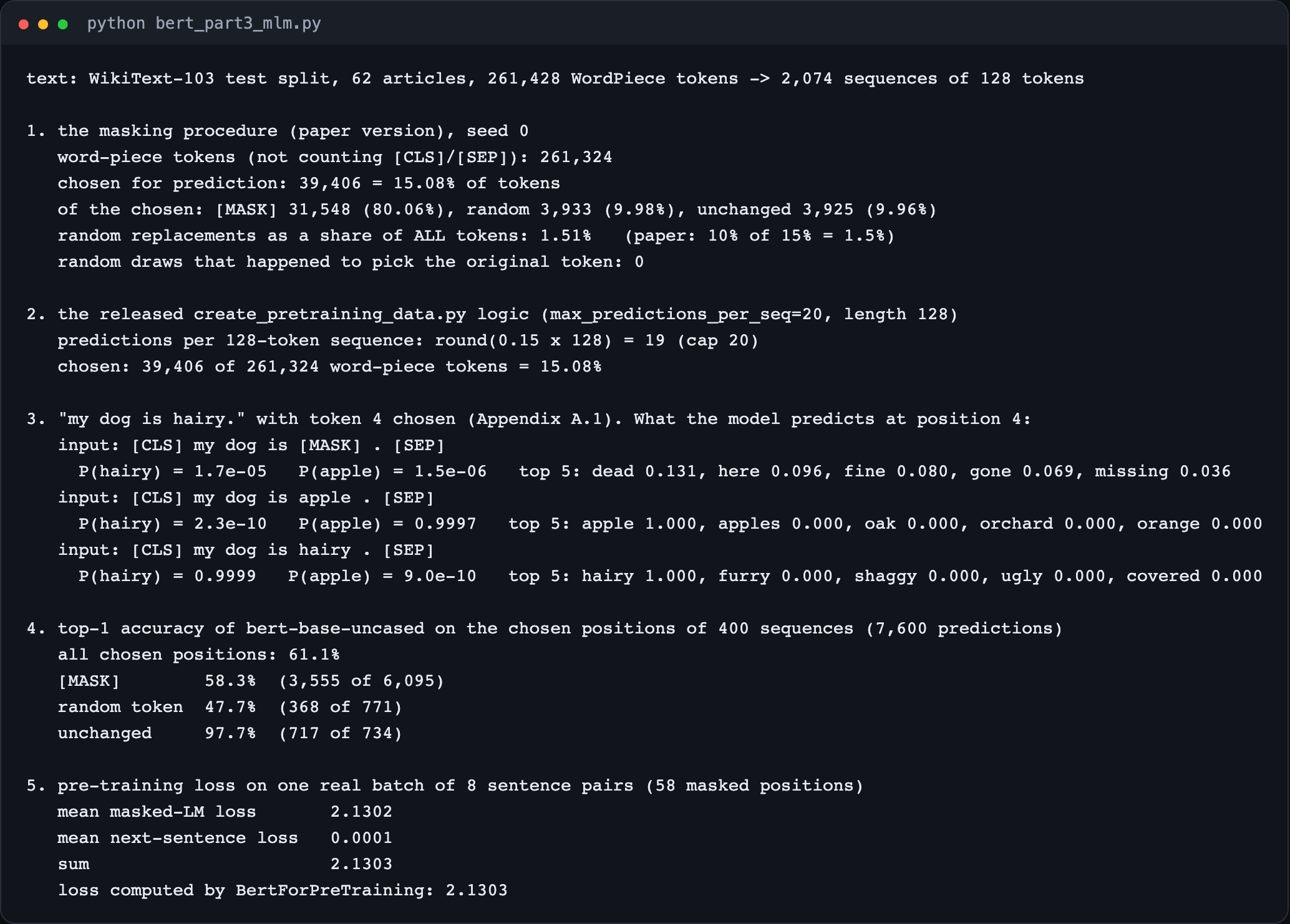
I ran it over the whole test split of WikiText-103 (62 Wikipedia articles), cut into sequences of 128 WordPiece tokens, with a fixed random seed:

1. the masking procedure (paper version), seed 0
   word-piece tokens (not counting [CLS]/[SEP]): 261,324
   chosen for prediction: 39,406 = 15.08% of tokens
   of the chosen: [MASK] 31,548 (80.06%), random 3,933 (9.98%), unchanged 3,925 (9.96%)
   random replacements as a share of ALL tokens: 1.51%   (paper: 10% of 15% = 1.5%)

How does this compare with Google's released code (create_pretraining_data.py in the BERT repository)? I read it line by line. It does the same thing, with three small differences that the paper does not mention:

• It picks an exact count per sequence, $\text{round}(0.15 \times \text{length})$, which for 128 tokens is 19. Re-running its logic on the same text chose exactly the same number of tokens as above, 39,406.
• It has a cap, max_predictions_per_seq (20 in the README's example for length 128). The README says to set it to about length × 15%, so the cap and the rate agree.
• It never masks [CLS] or [SEP], and the random replacement is drawn from the whole vocabulary file, special tokens included.

"my dog is hairy" on the real model#

Now the three cases of Appendix A.1, on the real bert-base-uncased. One honest change: the paper writes the sentence without a full stop. Without it, the model spends its guess at position 4 on the missing full stop (real sentences end with punctuation), so I added one.

3. "my dog is hairy." with token 4 chosen (Appendix A.1). What the model predicts at position 4:
   input: [CLS] my dog is [MASK] . [SEP]
     P(hairy) = 1.7e-05   P(apple) = 1.5e-06   top 5: dead 0.131, here 0.096, fine 0.080, gone 0.069, missing 0.036
   input: [CLS] my dog is apple . [SEP]
     P(hairy) = 2.3e-10   P(apple) = 0.9997   top 5: apple 1.000, apples 0.000, oak 0.000, orchard 0.000, orange 0.000
   input: [CLS] my dog is hairy . [SEP]
     P(hairy) = 0.9999   P(apple) = 9.0e-10   top 5: hairy 1.000, furry 0.000, shaggy 0.000, ugly 0.000, covered 0.000

This short example teaches more than it seems:

• [MASK]: "hairy" gets a probability of only 0.000017. That is correct behaviour: nothing in "my dog is ___." points to "hairy". The model offers sensible guesses ("dead", "here", "fine").
• Random word: the model believes "apple" (0.9997). In a four-word sentence there is no context to overrule it, and in pre-training only 1.5% of all tokens were random replacements, so a visible word is almost always the real one.
• Unchanged: "hairy" gets 0.9999. This is the "bias towards the actual observed word" that the appendix describes.

How often does BERT recover the original word?#

On a short sentence the model has little to go on. On real paragraphs it has a lot. I masked 400 of the 128-token sequences above with the same procedure and checked how often the real model's top guess is the original token:

4. top-1 accuracy of bert-base-uncased on the chosen positions of 400 sequences (7,600 predictions)
   all chosen positions: 61.1%
   [MASK]        58.3%  (3,555 of 6,095)
   random token  47.7%  (368 of 771)
   unchanged     97.7%  (717 of 734)

With a whole paragraph of context, BERT finds the hidden word 58.3% of the time, out of 30,522 possible tokens. And it corrects almost half of the random replacements (47.7%), which is exactly the skill the 10% random case trains. One caution: WikiText is made of Wikipedia articles, and BERT was pre-trained on Wikipedia, so the model may have seen some of this text. These numbers show the mechanism, not a clean test score.

The cost: only 15% of tokens teach anything#

Task 2: next sentence prediction#

Here is where NSP lives in the paper's Figure 1: the left-most output, $C$, feeds the box marked NSP.

The NSP loss is cross-entropy over two classes:

where:

• $y$ is the true label, IsNext or NotNext;
• $C$ is the final vector of [CLS], with 768 numbers in BERT-base;
• $W_{\text{NSP}}$ is a small learned matrix with 2 rows (one score per class) and 768 columns.

(In the released model, $C$ first passes through one extra layer, called the pooler, a 768-by-768 dense layer with a tanh function, and the classifier has a bias. The idea is the same.)

Appendix A.1 shows two examples:

The real NSP head#

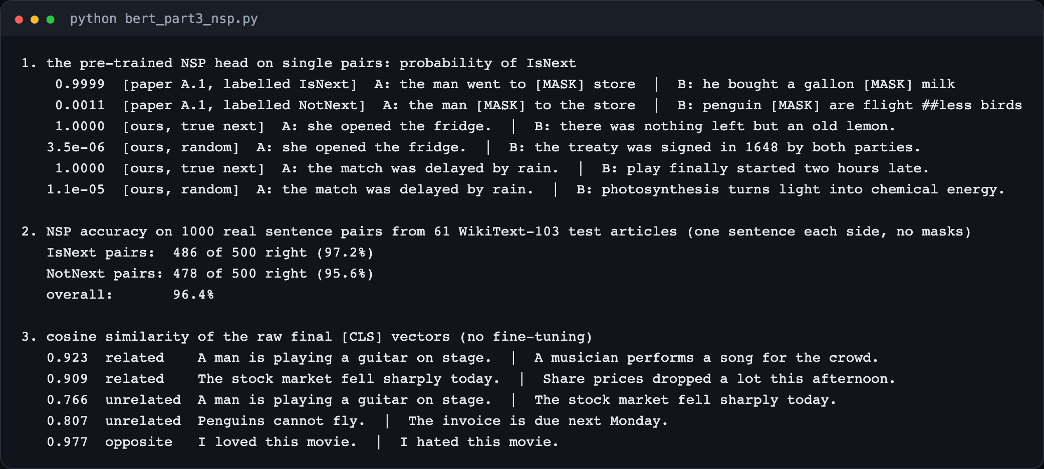
The released bert-base-uncased still contains its trained NSP layer, so we can ask it. Here are the paper's two examples and four pairs of my own:

1. the pre-trained NSP head on single pairs: probability of IsNext
    0.9999  [paper A.1, labelled IsNext]  A: the man went to [MASK] store  |  B: he bought a gallon [MASK] milk
    0.0011  [paper A.1, labelled NotNext]  A: the man [MASK] to the store  |  B: penguin [MASK] are flight ##less birds
    1.0000  [ours, true next]  A: she opened the fridge.  |  B: there was nothing left but an old lemon.
   3.5e-06  [ours, random]  A: she opened the fridge.  |  B: the treaty was signed in 1648 by both parties.
    1.0000  [ours, true next]  A: the match was delayed by rain.  |  B: play finally started two hours late.
   1.1e-05  [ours, random]  A: the match was delayed by rain.  |  B: photosynthesis turns light into chemical energy.

All six are right, and very confident. The paper reports how good the final model is in a footnote:

The NSP head, worked by hand. In the released model, $C$ first passes through the pooler (Part 2), then a two-way linear classifier:

where $W_p$ is $768 \times 768$, $W$ is $2 \times 768$ (one row per class: row 0 IsNext, row 1 NotNext), $s = (s_0, s_1)$ are the two scores, and $\tanh$ squeezes every number into the range -1 to 1. The loss is $-\log$ of the right class's probability. On the paper's two Appendix A.1 examples:

A: the man went to [MASK] store | B: he bought a gallon [MASK] milk | label IsNext
  scores W C + b = [5.111, -4.188]   (library: [5.111, -4.188])
  softmax: P(IsNext) = 0.999908, P(NotNext) = 0.000092; loss -log P(IsNext) = 0.000092
A: the man [MASK] to the store | B: penguin [MASK] are flightless birds | label NotNext
  scores W C + b = [-2.080, 4.691]   (library: [-2.080, 4.691])
  softmax: P(IsNext) = 0.001145, P(NotNext) = 0.998855; loss -log P(NotNext) = 0.001146

For the first pair, the gap between the two scores is $5.111 - (-4.188) = 9.299$, so

(A two-way softmax only depends on the difference of the two scores, which is why it can be written with a single exponential.)

2. NSP accuracy on 1000 real sentence pairs from 61 WikiText-103 test articles (one sentence each side, no masks)
   IsNext pairs:  486 of 500 right (97.2%)
   NotNext pairs: 478 of 500 right (95.6%)
   overall:       96.4%

96.4% is close to the paper's 97% to 98%, but the two numbers are not the same test. The paper does not say what data its figure comes from, and its "sentences" are long spans of text, while mine are single sentences cut by a simple splitter. Treat it as "the same ballpark", nothing more. Note also that a random sentence from another article is usually about a different topic, which makes NotNext easy to spot. Part 6 comes back to this.

Checking footnote 6. If $C$ were a good summary of a sentence's meaning, similar sentences would get similar vectors. I compared the raw $C$ vectors with cosine similarity:

3. cosine similarity of the raw final [CLS] vectors (no fine-tuning)
   0.923  related    A man is playing a guitar on stage.  |  A musician performs a song for the crowd.
   0.909  related    The stock market fell sharply today.  |  Share prices dropped a lot this afternoon.
   0.766  unrelated  A man is playing a guitar on stage.  |  The stock market fell sharply today.
   0.807  unrelated  Penguins cannot fly.  |  The invoice is due next Monday.
   0.977  opposite   I loved this movie.  |  I hated this movie.

Every pair scores above 0.76, and the two sentences with opposite meanings score highest of all (0.977). Related pairs do score a bit higher than unrelated ones, but the gaps are small and unreliable. Footnote 6 is right: without fine-tuning, $C$ is not a meaning vector. (Part 6 shows models fine-tuned specially to fix this.)

NSP and earlier work#

The two cited papers, in their own words:

The pre-training data#

What is in the BooksCorpus? Its paper (Zhu et al., 2015) describes it:

And the Billion Word Benchmark, which the paper rules out, says this about itself:

The pre-training procedure#

Appendix A.2 gives the exact recipe. First, how one training example is built.

Google noticed this too. In May 2019 the BERT repository added Whole Word Masking models (its README: "New May 31st, 2019: Whole Word Masking Models"), which always mask every piece of a word together. The released masking code has a switch for it, and its comment notes that the training itself does not change: each piece is still predicted on its own.

Next, the training run itself. The sentence starts at the bottom of the left column:

The batch and the 40 epochs#

Let us check the arithmetic (real output of bert_part3_schedule.py):

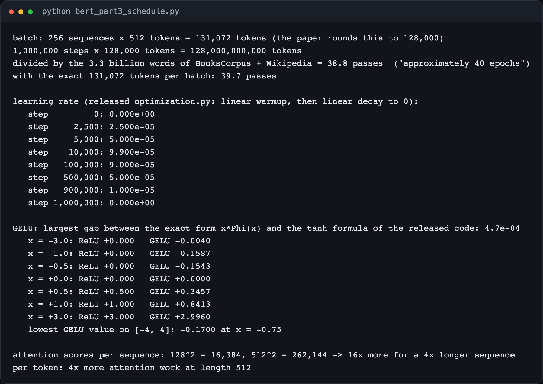
batch: 256 sequences x 512 tokens = 131,072 tokens (the paper rounds this to 128,000)
1,000,000 steps x 128,000 tokens = 128,000,000,000 tokens
divided by the 3.3 billion words of BooksCorpus + Wikipedia = 38.8 passes  ("approximately 40 epochs")
with the exact 131,072 tokens per batch: 39.7 passes

So "approximately 40 epochs" checks out. Two honest caveats about this calculation, both from the paper itself. It divides tokens by words, and WordPiece makes slightly more tokens than words. And it assumes every step uses 512 tokens, but (as we will see in a moment) 90% of the steps used sequences of 128 tokens, and the paper does not say what batch size was used then. So the true number of tokens seen is not stated anywhere in the paper; "about 40 epochs" is the paper's own rough figure.

Adam, warmup and decay#

The released code (optimization.py) computes the learning rate at step $s$ like this:

where $\eta$ (the Greek letter "eta") is the learning rate, $\eta_{\max} = 10^{-4}$ is the peak from the paper, and $s$ is the step number.

A small detail you only see in code: the decay is counted from step 0, so when warmup ends at step 10,000 the rate is already $10^{-4} \times 0.99 = 9.9 \times 10^{-5}$, not quite the peak.

The paper calls it "L2 weight decay". The released optimizer does not add a squared-weight penalty to the loss (a code comment explains that this interacts badly with Adam). Instead it subtracts a small fraction of each weight directly at every update, and it skips LayerNorm weights and biases. This later became known as decoupled weight decay, the "W" in the name of the AdamW optimizer.

GELU instead of ReLU#

The usual choice was ReLU, which keeps positive numbers and turns negative ones into 0. BERT uses GELU (Hendrycks and Gimpel, 2016), as OpenAI GPT did:

where:

• $x$ is the input number;
• $\Phi(x)$ (the Greek letter "phi") is the probability that a random number from a standard bell curve (a normal distribution with mean 0 and spread 1) is smaller than $x$. It goes smoothly from 0 (for very negative $x$) to 1 (for very positive $x$).

So GELU keeps $x$ in proportion to how large $x$ is. Big positive inputs pass almost unchanged, big negative inputs become almost 0, and small inputs are scaled down smoothly.

$\Phi$ has no simple closed form, so the released code uses a fast approximation based on tanh:

where $\operatorname{erf}$ is the "error function" of statistics. Worked values:

x = -1.0: Phi(x) = 0.1587, GELU = -1.0 x 0.1587 = -0.1587; tanh formula -0.1588; ReLU +0.0
x = -0.5: Phi(x) = 0.3085, GELU = -0.5 x 0.3085 = -0.1543; tanh formula -0.1543; ReLU +0.0
x = +0.5: Phi(x) = 0.6915, GELU = +0.5 x 0.6915 = +0.3457; tanh formula +0.3457; ReLU +0.5
x = +1.0: Phi(x) = 0.8413, GELU = +1.0 x 0.8413 = +0.8413; tanh formula +0.8412; ReLU +1.0

Read the $x = +0.5$ row: a standard bell-curve number is below 0.5 with probability 0.6915, so GELU lets 69% of the input through: $0.5 \times 0.6915 = 0.346$. ReLU would pass all of it.

GELU: largest gap between the exact form x*Phi(x) and the tanh formula of the released code: 4.7e-04
   x = -3.0: ReLU +0.000   GELU -0.0040
   x = -1.0: ReLU +0.000   GELU -0.1587
   x = -0.5: ReLU +0.000   GELU -0.1543
   x = +0.0: ReLU +0.000   GELU +0.0000
   x = +0.5: ReLU +0.500   GELU +0.3457
   x = +1.0: ReLU +1.000   GELU +0.8413
   x = +3.0: ReLU +3.000   GELU +2.9960

The released code computes $\Phi$ with a fast formula based on tanh. It differs from the exact GELU by at most 0.00047.

One loss for both tasks#

The training loss is the sum of the two tasks' average losses:

where $\mathcal{L}_{\text{MLM}}$ is the mean cross-entropy over all masked positions in the batch and $\mathcal{L}_{\text{NSP}}$ is the mean cross-entropy over all sentence pairs. (The paper says "likelihood"; training minimises the negative log-likelihood, which is the same cross-entropy.)

I checked this on a real batch: 8 sentence pairs from Wikipedia (half IsNext, half NotNext), masked with the procedure above, through BertForPreTraining:

5. pre-training loss on one real batch of 8 sentence pairs (58 masked positions)
   mean masked-LM loss       2.1302
   mean next-sentence loss   0.0001
   sum                       2.1303
   loss computed by BertForPreTraining: 2.1303

The two parts add up exactly to the loss the library computes. Notice how lopsided they are: next sentence prediction is nearly solved (0.0001), while filling in blanks is still hard (2.1302). After pre-training, almost all of the remaining learning signal comes from the masked LM.

The same check on the paper's own two Appendix A.1 examples, where every number can be followed:

pair 1, position  5, target "the": p = 0.8087, loss 0.2123
pair 1, position 12, target "of": p = 0.9986, loss 0.0014
pair 2, position  3, target "went": p = 0.0755, loss 2.5830
pair 2, position  9, target "##s": p = 0.0032, loss 5.7557
mean MLM loss over 4 masked positions: 2.1381
NSP loss per pair: 0.000092, 0.001146; mean 0.000619
total = 2.1381 + 0.000619 = 2.1387   (BertForPreTraining: 2.1387)

(The paper does not print the hidden words in A.1; the script restores the obvious ones. "##s" is the last piece of "penguins": its probability is low because, seeing "penguin [MASK]", the model mostly expects other continuations.)

Hardware and the two sequence lengths#

attention scores per sequence: 128^2 = 16,384, 512^2 = 262,144 -> 16x more for a 4x longer sequence
per token: 4x more attention work at length 512

The other parts of the model (the feed-forward layers) cost the same per token at any length, so attention is the part that blows up. Training mostly at length 128 saves a lot. But the position embeddings for positions 128 to 511 (Part 2) are only trained in the final 10% of steps, which is the reason for that last phase.

How big is the effect for BERT-base, exactly? Count multiply-adds per layer for a sequence of $n$ tokens with $H = 768$:

where the first term grows like $n$ (each token does the same matrix work) and the second like $n^2$ (every pair of tokens).

n = 128: projections + feed-forward 905,969,664; attention scores and mixing 25,165,824
         attention share of a layer's work: 2.7%; work per token 7,274,496
n = 512: projections + feed-forward 3,623,878,656; attention scores and mixing 402,653,184
         attention share of a layer's work: 10.0%; work per token 7,864,320
512 vs 128: score matrix 16x, whole-sequence work 4.32x (4x the tokens), work per token 1.08x

So the paper's statement is true (the $n^2$ part does grow 16-fold), but at $n \le 512$ it is a modest share of the total. The bigger practical costs of long sequences on 2018 hardware were memory (every layer stores $n \times n$ attention weights per head for the backward pass) and the 4 times larger batch in tokens. The short-then-long schedule saves time either way:

Next, in Part 4: fine-tuning. How the same pre-trained BERT becomes a classifier, a question-answering system and a multiple-choice solver, the paper's results tables, and a real fine-tuning run.

Run it yourself

The scripts behind every number in this part are in code/papers/bert/. They need Python with torch, transformers and datasets, and download bert-base-uncased (about 440 MB) and the WikiText data the first time.

bashCopy

pip install torch transformers datasets
python bert_part3_seeitself.py   # the three tiny models (about 6 minutes per model on a laptop GPU)
python bert_part3_mlm.py         # masking statistics, "my dog is hairy", MLM accuracy, the loss on a batch
python bert_part3_nsp.py         # the NSP head, 1,000 real pairs, raw [CLS] similarities
python bert_part3_schedule.py    # batch arithmetic, learning rate, GELU, attention cost

References#

The BERT paper

1. J. Devlin, M.-W. Chang, K. Lee, K. Toutanova. BERT: Pre-training of Deep Bidirectional Transformers for Language Understanding. NAACL 2019 (ACL Anthology).
2. Google Research. BERT code and models, including create_pretraining_data.py, run_pretraining.py, optimization.py and the Whole Word Masking models.

Papers the BERT paper cites in this part

3. W. L. Taylor. "Cloze Procedure": A New Tool for Measuring Readability. Journalism Quarterly 30(4), 1953.
4. P. Vincent, H. Larochelle, Y. Bengio, P.-A. Manzagol. Extracting and composing robust features with denoising autoencoders. ICML 2008.
5. Y. Jernite, S. R. Bowman, D. Sontag. Discourse-Based Objectives for Fast Unsupervised Sentence Representation Learning. arXiv 2017.
6. L. Logeswaran, H. Lee. An efficient framework for learning sentence representations. ICLR 2018.
7. Y. Zhu, R. Kiros, R. Zemel, R. Salakhutdinov, R. Urtasun, A. Torralba, S. Fidler. Aligning Books and Movies: Towards Story-like Visual Explanations by Watching Movies and Reading Books (BooksCorpus). ICCV 2015.
8. C. Chelba, T. Mikolov, M. Schuster, Q. Ge, T. Brants, P. Koehn, T. Robinson. One Billion Word Benchmark for Measuring Progress in Statistical Language Modeling. arXiv 2013.
9. D. Hendrycks, K. Gimpel. Gaussian Error Linear Units (GELUs). arXiv 2016.
10. A. Radford, K. Narasimhan, T. Salimans, I. Sutskever. Improving Language Understanding by Generative Pre-Training (OpenAI GPT, which also used GELU and the BooksCorpus). OpenAI, 2018.

Other sources used in this part

11. S. Merity, C. Xiong, J. Bradbury, R. Socher. Pointer Sentinel Mixture Models (the WikiText data used in our measurements). ICLR 2017.
12. Code for this part: bert_part3_seeitself.py, bert_part3_mlm.py, bert_part3_nsp.py, bert_part3_schedule.py, bert_part3_math.py.