BERT, explained · Part 2 of 6 · Covers §2, §3 (model, input)

Inside BERT: Architecture and Input

Section 2 and the model half of Section 3, line by line: the ideas BERT builds on, the stack of Transformer layers, where the 110 million parameters come from (counted in the real model), WordPiece tokens, [CLS], [SEP], and the three embeddings that are added together for every token.

BERT: Pre-training of Deep Bidirectional Transformers for Language Understanding. Jacob Devlin, Ming-Wei Chang, Kenton Lee, Kristina Toutanova. NAACL 2019, 2018. arXiv:1810.04805

In Part 1 we read the paper's big idea: pre-train a Transformer that looks at both sides of every word, then fine-tune it. This part opens the box. First we read Section 2, the history BERT builds on. Then the first half of Section 3: what the model is made of, how big it is, and how text is turned into the numbers it reads.

Everything that can be checked, we check on the real released model, bert-base-uncased.

The three groups are: feature-based approaches (§2.1), fine-tuning approaches (§2.2), and transfer from labelled data (§2.3). We take them one at a time.

The related work on one timeline. Feature-based methods (word2vec, GloVe, skip-thought, ELMo) produce frozen vectors for another model. Fine-tuning methods (Collobert and Weston, Dai and Le, ULMFiT, OpenAI GPT) keep training the whole pre-trained network. Labelled transfer (ImageNet, InferSent, CoVe) pre-trains on a big labelled task. BERT takes the fine-tuning recipe and the ImageNet habit, with unlabeled text.

Word embeddings

A word embedding is a lookup table: one row per word. The word "bank" always gets the same row, whether it is a river bank or a money bank. Keep this weakness in mind; the next two paragraphs are about fixing it.

Three generations of word representations. Non-neural: Brown clusters (1992) give each word a code from a tree of word groups built from counts. Neural, static: word2vec and GloVe learn one vector per word. Contextual: ELMo and BERT compute a new vector for every sentence.

The paragraph says word vectors were trained with left-to-right language models and with objectives that "discriminate correct from incorrect words in left and right context". The second phrase is word2vec. Here is its picture and its training objective, from its own papers:

The objective, symbol by symbol:

\log \sigma\!\left(v'^{\top}_{w_O} v_{w_I}\right) + \sum_{i=1}^{k} \mathbb{E}_{w_i \sim P_n(w)}\!\left[\log \sigma\!\left(-v'^{\top}_{w_i} v_{w_I}\right)\right]

where:

$w_I$ is the input (centre) word and $w_O$ a real word from its window; $v_{w_I}$ and $v'_{w_O}$ are their vectors (word2vec keeps two vectors per word, one for each role);
$\sigma(x) = 1 / (1 + e^{-x})$ is the sigmoid, which squeezes any number into a probability between 0 and 1;
the first term is large when the real pair's dot product is large ("these two go together");
$w_1, \dots, w_k$ are $k$ random words drawn from a noise distribution $P_n(w)$ (common words drawn more often); the second term is large when their dot products with the centre word are very negative ("these do not go together");
$\mathbb{E}$ means "on average over the random draws". Training makes the whole expression as large as possible.

The skip-gram setup on "the cat sat on the mat". The centre word "sat" has a window of two words on each side. Training pairs it with its real neighbours (target 1) and with random words such as "banana" (target 0), and learns vectors so that sigmoid of the dot product tells them apart.

Sentence and paragraph embeddings

The paragraph packs three earlier sentence objectives into one sentence. Each one is a small idea worth seeing, because BERT borrows from two of them.

1. Generate the neighbouring sentences (skip-thought). Kiros et al. (2015) encode a sentence into one vector, then train two decoders to write the sentence before it and the sentence after it.

2. Rank candidate next sentences. Jernite et al. (2017) and Logeswaran and Lee (2018) skip the writing. They give the model a sentence and a few candidates, and train it to pick the one that really came next.

3. Repair a damaged sentence (denoising auto-encoders). Hill et al. (2016) corrupt a sentence and train an encoder-decoder to rebuild the original.

Learning sentence vectors from neighbouring sentences. Skip-thought writes the previous and next sentence from one sentence vector. Ranking methods score candidate sentences and pick the true next one (scores here are an illustration).

Denoising, step by step. A clean sentence is damaged (a word deleted, two words swapped). An SDAE rebuilds every word of the original. BERT's masked LM hides one word and predicts only that word.

ELMo: a word's vector depends on its sentence

From the paperDevlin et al. (2018), BERTSection 2.1page 2

Where this is

The third paragraph of Section 2.1, about the strongest feature-based model of 2018.

What it says

ELMo extracts "context-sensitive features" from a left-to-right and a right-to-left language model. Each token's vector "is the concatenation of the left-to-right and right-to-left representations". Plugged into existing task models, ELMo set new records in question answering, sentiment analysis and named entity recognition. Melamud et al. (2016, called context2vec) predicted a word from both sides with LSTMs, but, like ELMo, it is "not deeply bidirectional". Fedus et al. (2018) used the Cloze task to improve text generation.

Why it matters

ELMo fixed the "bank" problem: the vector of a word now depends on its sentence. BERT keeps that, and makes the two directions mix in every layer instead of only at the end.

ELMo's vector for "bank", drawn. A left-to-right LSTM and a right-to-left LSTM each read the sentence on their own. The vector for "bank" is the forward state glued to the backward state. Inside each reader, information flows one way only.

We can see the difference between a static and a contextual vector in the real BERT. BERT has both kinds inside it: its first step is a lookup table (a static embedding, one row per token), and its output is a contextual vector. I took the word "bank" in four sentences, two about rivers and two about money, and compared the vectors with cosine similarity.

As a formula, for two vectors $a$ and $b$ of the same length:

\cos(a, b) = \frac{a \cdot b}{\lVert a \rVert \, \lVert b \rVert}, \qquad a \cdot b = \sum_i a_i b_i, \qquad \lVert a \rVert = \sqrt{\textstyle\sum_i a_i^2}

where $a \cdot b$ is the dot product and $\lVert a \rVert$ the length. A tiny example: $a = (1, 2, 2)$ and $b = (2, 1, 2)$ give $a \cdot b = 2 + 2 + 4 = 8$ , $\lVert a \rVert = \lVert b \rVert = 3$ , so $\cos = 8 / 9 = 0.889$ . BERT's vectors have 768 numbers instead of 3, but the formula is the same.

python

import torch, torch.nn.functional as F
from transformers import BertModel, BertTokenizer

tok = BertTokenizer.from_pretrained("bert-base-uncased")
model = BertModel.from_pretrained("bert-base-uncased").eval()

def bank_vector(sentence):
    enc = tok(sentence, return_tensors="pt")
    pos = enc.input_ids[0].tolist().index(tok.vocab["bank"])   # where "bank" is
    return model(**enc).last_hidden_state[0, pos]              # BERT's output vector for it (768 numbers)

a = bank_vector("he sat on the river bank and watched the water.")
b = bank_vector("she opened a savings account at the bank.")
print(F.cosine_similarity(a, b, dim=0))

The real output, for all four sentences:

plain text

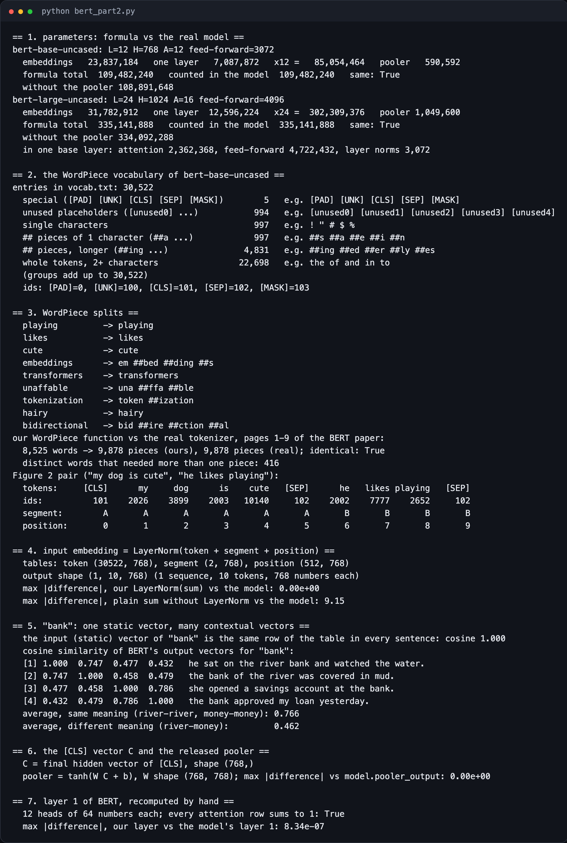
the input (static) vector of "bank" is the same row of the table in every sentence: cosine 1.000
cosine similarity of BERT's output vectors for "bank":
[1] 1.000  0.747  0.477  0.432   he sat on the river bank and watched the water.
[2] 0.747  1.000  0.458  0.479   the bank of the river was covered in mud.
[3] 0.477  0.458  1.000  0.786   she opened a savings account at the bank.
[4] 0.432  0.479  0.786  1.000   the bank approved my loan yesterday.
average, same meaning (river-river, money-money): 0.766
average, different meaning (river-money):         0.462

Cosine similarity of BERT's output vectors for "bank". The two river sentences are close (0.747), the two money sentences are close (0.786), and every river and money pair is far apart (0.432 to 0.479). A static word embedding would give 1.000 everywhere.

The static row of the table cannot tell the two banks apart: it is literally the same vector. After 12 layers of looking at the neighbours, BERT's output vectors split cleanly into a "river" group and a "money" group. This is what "contextual" means, and it is what made ELMo, and then BERT, so useful.

Use case. A search engine that knows "bank" in "fishing spots on the river bank" is not about money will not show loan offers for that query.

Fine-tuning approaches

From the paperDevlin et al. (2018), BERTSection 2.2pages 2 and 3

Where this is

Section 2.2, the family BERT belongs to. It runs from page 2 onto page 3.

What it says

The first works (Collobert and Weston, 2008) "only pre-trained word embedding parameters". Later, whole encoders were pre-trained on unlabeled text and "fine-tuned for a supervised downstream task" (Dai and Le, 2015; Howard and Ruder, 2018; Radford et al., 2018). The advantage: "few parameters need to be learned from scratch". This is partly why OpenAI GPT held the previous best results on many GLUE tasks. They were pre-trained with left-to-right language modelling and auto-encoder objectives.

Why it matters

BERT takes this recipe unchanged (pre-train everything, fine-tune everything) and only changes what happens during pre-training.

The key phrase is "few parameters need to be learned from scratch". With the feature-based approach, the whole task model above the features starts from random numbers and must learn from the task's small labelled set. With fine-tuning, almost every weight starts pre-trained; only a tiny output layer is new. Less to learn from scratch means less labelled data is needed. Howard and Ruder's 2018 paper (ULMFiT) showed this works well for text classification with LSTMs; GPT showed it with a Transformer.

Transfer learning from labelled data

The transfer-learning recipe in vision and in language. Step 1, done once: pre-train a big network on a huge dataset (ImageNet's 1.2 million labelled photos; BERT's 3.3 billion words of unlabeled text). Step 2, done for every new task: start from a copy of those weights and fine-tune.

BERT in two steps, with one architecture

Now Section 3, the description of BERT itself. It opens with the two steps and with the paper's main picture, Figure 1.

How to read Figure 1, from bottom to top:

Bottom (pink): the input tokens. [CLS], then the tokens of sentence A (Tok 1 to Tok N), then [SEP], then the tokens of sentence B (Tok 1 to Tok M).
Yellow: E, the input embedding of each token. We build these by hand later in this part.
Blue box: BERT itself, the stack of layers. Every position is connected to every other (the faint lines).
Green (top): the outputs. C is the output for [CLS]. T₁, …, T_N and T₁′, …, T_M′ are the outputs for the other tokens.
Red arrows (top): the output layers. In pre-training, C feeds NSP (next sentence prediction) and the T vectors feed Mask LM. In fine-tuning, the output layer depends on the task: for SQuAD (question answering), the T vectors of the paragraph predict where the answer starts and ends.

Figure 1 redrawn with real words. Left, pre-training: "[CLS] my [MASK] [SEP] he [MASK] [SEP]"; C feeds the IsNext question, the T vectors at the masked positions predict "dog" and "likes". Right, fine-tuning on SQuAD: a question and a paragraph go through the same encoder, starting from the same weights, and the paragraph's T vectors predict where the answer "Ada" starts and ends. C is unused there.

The model: a stack of Transformer encoder layers

The paper skips the details of the Transformer and points to Vaswani et al. (2017) and the guide "The Annotated Transformer". Here is the short version, enough to follow the rest of the paper.

Every BERT layer has the same two parts:

Self-attention with A heads: each token gathers information from the other tokens.
A feed-forward network: each token's vector is processed on its own by two matrix multiplications with a non-linear step between them.

After each part there is an add-and-normalise step: the part's output is added to its input (a "residual connection"), then normalised with LayerNorm. Written as equations, for the vectors $h$ of all tokens entering a layer:

h' = \text{LayerNorm}\big(h + \text{MultiHeadAttention}(h)\big)

\text{output} = \text{LayerNorm}\big(h' + \text{FFN}(h')\big), \qquad \text{FFN}(x) = \text{GELU}(x W_1 + b_1)\, W_2 + b_2

where:

$h$ holds one $H$ -number vector per token (the input of the layer), and $h'$ is the result after attention;
$\text{MultiHeadAttention}$ runs $A$ attention heads in parallel and joins their results;
$W_1$ is an $H \times 4H$ matrix and $W_2$ a $4H \times H$ matrix, with bias vectors $b_1$ and $b_2$ : the feed-forward network makes each vector four times wider, then narrows it back;
$\text{GELU}$ is a smooth version of "keep positive numbers, set negative ones to zero" (Part 3 shows its shape);
$\text{LayerNorm}$ rescales each vector to have mean 0 and spread 1, then applies a learned scale and shift.

The paper hands the details to Vaswani et al. and to "The Annotated Transformer" in two footnotes:

Inside one layer: attention, with real numbers

The heart of each layer is the attention equation of Vaswani et al.:

Where do $Q$ , $K$ and $V$ come from? Each is the layer input $X$ (one row of $H = 768$ numbers per token) multiplied by a learned matrix:

Q = X W^Q, \qquad K = X W^K, \qquad V = X W^V, \qquad \text{head} = \operatorname{softmax}\!\left(\frac{QK^\top}{\sqrt{d_k}}\right) V

where, for one head of BERT-base and a text of $n$ tokens:

$X$ is $n \times 768$ ;
$W^Q$ , $W^K$ , $W^V$ are each $768 \times 64$ , so $Q$ , $K$ , $V$ are $n \times 64$ (here $d_k = 64$ );
$QK^\top$ is $n \times n$ : one score for every pair of tokens;
softmax works row by row, so each row of weights adds up to 1;
multiplying by $V$ gives the head's output, $n \times 64$ : for each token, a weighted mix of all tokens' value rows.

One attention head of BERT-base, shape by shape, for a text of n tokens. X (n × 768) times W_Q (768 × 64) gives Q (n × 64); the same for K and V. Q times Kᵀ gives an n × n table of scores; divided by 8 and passed through softmax, it becomes weights; the weights times V give the head's output Z (n × 64).

A worked example small enough to check by hand. Three tokens, $d_k = 4$ , with simple numbers chosen for the example (bert_part2_math.py):

plain text

Q K^T:
  the      1.000  0.000  2.000
  kid      0.000  3.000  2.000
  smiles   1.000  2.000  3.000
/ sqrt(d_k):
  the      0.500  0.000  1.000
  kid      0.000  1.500  1.000
  smiles   0.500  1.000  1.500
softmax:
  the      0.307  0.186  0.506
  kid      0.122  0.547  0.331
  smiles   0.186  0.307  0.506
output = weights V:
  the      0.814  0.693
  kid      0.453  0.878
  smiles   0.693  0.814
row sums of the weights: [1.0, 1.0, 1.0]

Check the row for "kid": the scaled scores are 0, 1.5 and 1.0, and

\frac{e^{0}}{e^{0} + e^{1.5} + e^{1.0}} = \frac{1}{1 + 4.482 + 2.718} = \frac{1}{8.200} = 0.122

and likewise $4.482 / 8.200 = 0.547$ and $2.718 / 8.200 = 0.331$ . "kid" looks mostly at itself, then at "smiles", and all three weights add up to 1.

The tiny example as a picture. Left: the scaled scores. Middle: softmax turns each row into weights that add up to 1. Right: each token's output is the weighted mix of the value rows.

Why divide by $\sqrt{d_k}$ ? If the numbers in $q$ and $k$ are random with spread 1, their dot product (a sum of $d_k$ products) has spread about $\sqrt{d_k}$ . With $d_k = 64$ that is 8, and softmax over numbers that large picks one key and ignores the rest. Measured:

plain text

10,000 random pairs, each number drawn with mean 0 and spread 1
spread (standard deviation) of q.k:          8.002   (about sqrt(64) = 8)
spread of q.k / sqrt(64):                     1.000
softmax WITHOUT the division (scores x 8):    [ 0.530,  0.023,  0.004,  0.385,  0.000,  0.001,  0.000,  0.057]   max 0.530
softmax WITH the division:                    [ 0.208,  0.140,  0.114,  0.199,  0.068,  0.091,  0.023,  0.157]   max 0.208

The same eight scores through softmax, without and with the division by 8. Without it, one key takes 0.53 and three get almost nothing, so learning stalls. With it, the weights stay spread out and every key still gets some signal.

Many heads. One head learns one way of looking. BERT-base runs $A = 12$ heads side by side, each with its own $W^Q, W^K, W^V$ of $768 \times 64$ , and joins their outputs:

\text{MultiHead}(X) = \text{Concat}(\text{head}_1, \dots, \text{head}_A)\, W^O

where each $\text{head}_i$ is $n \times 64$ , the concatenation is $n \times 768$ , and $W^O$ is $768 \times 768$ .

Multi-head attention in BERT-base. Twelve heads, each producing 64 numbers per token, are joined side by side into 768 numbers and mixed by W_O (768 × 768).

Here is a real head of the real model on "the kid smiles":

plain text

tokens: ['[CLS]', 'the', 'kid', 'smiles', '[SEP]']  (n = 5)
X (input embeddings) (5, 768);  W_Q (768, 768) holds 12 heads of 64 columns
per head: Q (5, 64), K (5, 64), V (5, 64); Q K^T (5, 5); output (5, 64)
12 heads joined: (5, 768); after W_O (768, 768): (5, 768)
head 1 of layer 1, attention weights:
             [CLS]     the     kid  smiles   [SEP]
  [CLS]      0.108   0.246   0.063   0.076   0.506
  the        0.198   0.212   0.175   0.217   0.198
  kid        0.152   0.088   0.139   0.281   0.340
  smiles     0.144   0.160   0.185   0.235   0.276
  [SEP]      0.189   0.200   0.091   0.171   0.348

Head 1 of layer 1 of the real bert-base-uncased. Every square is allowed (no mask) and every row adds up to 1. "kid" looks most at [SEP] (0.340) and at "smiles" (0.281), the word on its right.

Inside one layer: the feed-forward network

The feed-forward network for one token. "kid" (768 numbers after attention) is widened to 3,072 by W₁, passed through GELU, and narrowed back to 768 by W₂. The same weights are used for every position in the layer. In this real example only 5.2% of the 3,072 numbers were positive before GELU.

Real numbers, for "kid" in layer 1:

plain text

in (768,) -> x W1 + b1 (3072,) -> GELU -> x W2 + b2 (768,)
first 6 of the 3072 numbers before GELU: [-1.334, -0.569, -4.067, -1.991, -1.904, -0.816]
the same 6 after GELU:                   [-0.122, -0.162, -0.000, -0.046, -0.054, -0.169]
share of the 3072 that are positive before GELU: 0.052

Negative inputs come out of GELU small but not exactly zero (-1.334 becomes -0.122), unlike ReLU, which would make them all 0. Very negative inputs (-4.067) do become almost exactly 0.

The BERT-base encoder. Tokens become input embeddings, go up through 12 identical layers (each with 12-head self-attention and a feed-forward network), and come out as one 768-number vector per token: C for [CLS] and T for every other token.

To check that this short description is complete, I recomputed layer 1 of the real bert-base-uncased by hand, using only its weights and the equations above:

python

x = model.embeddings(input_ids=ids, token_type_ids=seg)[0]     # (10 tokens, 768)
lay = model.encoder.layer[0]
A, d = 12, 64                                                  # 12 heads of 64 numbers
q = lay.attention.self.query(x).view(-1, A, d).transpose(0, 1) # (12, 10, 64)
k = lay.attention.self.key(x).view(-1, A, d).transpose(0, 1)
v = lay.attention.self.value(x).view(-1, A, d).transpose(0, 1)
att = torch.softmax(q @ k.transpose(1, 2) / d ** 0.5, dim=-1)  # no mask: both directions
heads = (att @ v).transpose(0, 1).reshape(-1, 768)             # join the 12 heads
h1 = lay.attention.output.LayerNorm(x + lay.attention.output.dense(heads))
out = lay.output.LayerNorm(h1 + lay.output.dense(F.gelu(lay.intermediate.dense(h1))))

plain text

== 7. layer 1 of BERT, recomputed by hand ==
  12 heads of 64 numbers each; every attention row sums to 1: True
  max |difference|, our layer vs the model's layer 1: 8.34e-07

The largest difference from the model's own layer is $8.34 \times 10^{-7}$ , the size of normal rounding errors in 32-bit arithmetic. So the equations above are the whole layer: attention, add and normalise, feed-forward, add and normalise.

Two model sizes: L, H and A

	Layers L	Hidden size H	Heads A	Numbers per head H/A	Feed-forward size 4H	Parameters (paper)
BERT-base	12	768	12	64	3,072	110M
BERT-large	24	1,024	16	64	4,096	340M

The feed-forward size comes from a footnote:

And footnote 4 explains two names you will see everywhere:

The mask is easiest to see as a grid. Each row is a token doing the looking; each column a token being looked at.

Attention masks. In BERT (left) every square is allowed: every token can attend to every token. In GPT (right) the upper triangle is blocked, so each token attends only to itself and to the tokens on its left. That one triangle is the difference between an encoder and a decoder.

A model that can only look left can write text one token at a time, because it never needs the future. A model that looks both ways can understand text better, but cannot simply write the next word. That trade-off is why BERT is used for understanding tasks and GPT-style models for generation.

Where "110 million" comes from

The paper gives the parameter counts as rounded totals. We can rebuild them from L, H, A, the 4H footnote and the vocabulary size. Every count below is checked against the real model.

Embeddings. Three lookup tables of $H$ numbers per row, plus one LayerNorm (a scale and a shift, $2H$ ):

\underbrace{30{,}522 \times 768}_{\text{tokens}} + \underbrace{512 \times 768}_{\text{positions}} + \underbrace{2 \times 768}_{\text{segments}} + \underbrace{2 \times 768}_{\text{LayerNorm}} = 23{,}837{,}184

One layer. Attention has four $H \times H$ matrices (query, key, value, output), each with a bias of $H$ . The feed-forward network has an $H \times 4H$ matrix with bias $4H$ and a $4H \times H$ matrix with bias $H$ . Two LayerNorms add $4H$ :

\underbrace{4(H^2 + H)}_{\text{attention}} + \underbrace{2 \cdot 4H^2 + 4H + H}_{\text{feed-forward}} + \underbrace{4H}_{\text{2 LayerNorms}} = 2{,}362{,}368 + 4{,}722{,}432 + 3{,}072 = 7{,}087{,}872

where $H = 768$ . Twelve layers give $12 \times 7{,}087{,}872 = 85{,}054{,}464$ .

Pooler. One more $H \times H$ matrix with a bias, $H^2 + H = 590{,}592$ (more on it at the end of this part).

Total: $23{,}837{,}184 + 85{,}054{,}464 + 590{,}592 = 109{,}482{,}240$ .

The script computes the same formula and also counts every parameter in the downloaded model. For BERT-large, it builds the model's shape from its configuration file on PyTorch's "meta" device, which creates the layers without storing any weights, so nothing big is downloaded:

python

from transformers import BertConfig, BertModel
import torch

c = BertConfig.from_pretrained("bert-large-uncased")   # only the small config file
with torch.device("meta"):                             # shapes only, no memory used for weights
    large = BertModel(c)
print(sum(p.numel() for p in large.parameters()))

plain text

bert-base-uncased: L=12 H=768 A=12 feed-forward=3072
  embeddings   23,837,184   one layer   7,087,872   x12 =   85,054,464   pooler   590,592
  formula total  109,482,240   counted in the model  109,482,240   same: True
  without the pooler 108,891,648
bert-large-uncased: L=24 H=1024 A=16 feed-forward=4096
  embeddings   31,782,912   one layer  12,596,224   x24 =  302,309,376   pooler 1,049,600
  formula total  335,141,888   counted in the model  335,141,888   same: True
  without the pooler 334,092,288

Where BERT-base's 109,482,240 parameters live. The feed-forward networks hold about half (56.67 million), attention about a quarter (28.35 million), the embedding tables about a fifth (23.84 million).

The same count as bars, for BERT-base and BERT-large, with OpenAI GPT for comparison. In both BERTs the feed-forward networks are the biggest part. GPT has the same L, H and A as BERT-base, but 116.5 million parameters, mostly because its vocabulary is larger (40,478 tokens against 30,522).

So the formula and the real models agree exactly: 109,482,240 for BERT-base and 335,141,888 for BERT-large. The paper's "110M" and "340M" are both what you get by rounding these to the nearest 10 million (109.5 → 110, 335.1 → 340). The paper does not say how it rounded, so treat this as arithmetic, not as the authors' stated method.

Two things stand out in the picture:

The feed-forward networks are the biggest part, about 52% of all parameters. Making them 4H wide is expensive.
The token table alone is about a fifth of BERT-base: $30{,}522 \times 768 = 23{,}440{,}896$ numbers just to look up one vector per token. Later models (ALBERT, in Part 6) attack exactly this.

Input: sentences and sequences

WordPiece: how text becomes tokens

From the paperDevlin et al. (2018), BERTSection 3, Input/Output Representationspage 4

Where this is

The second paragraph of "Input/Output Representations". It is short but dense: five ideas in nine lines.

What it says

(1) "WordPiece embeddings (Wu et al., 2016) with a 30,000 token vocabulary". (2) Every sequence starts with [CLS], whose final vector is "the aggregate sequence representation for classification tasks". (3) Two sentences are separated by [SEP]. (4) A "learned embedding" on every token says whether it belongs to sentence A or B. (5) Names: E for input embeddings, $C \in \mathbb{R}^H$ for the final vector of [CLS], $T_i \in \mathbb{R}^H$ for the final vector of token $i$ .

Why it matters

These are the symbols used in every formula from here to the end of the paper.

We take the five ideas one at a time, starting with WordPiece.

Why not just use whole words? Because there are too many: names, typos, technical terms, word forms. A whole-word vocabulary would either be enormous or would map many words to "unknown". Why not single letters? Because sequences would get very long. WordPiece is the middle path: about 30,000 pieces cover everything.

The released tokenizer cuts each word with a simple rule, which its code comment calls "a greedy longest-match-first algorithm": take the longest piece at the start of the word that is in the vocabulary, then repeat on the rest with a ## in front. Here it is in a few lines of Python:

python

def wordpiece(word, vocab, unk="[UNK]"):
    pieces, start = [], 0
    while start < len(word):
        end = len(word)
        while end > start:                       # try the longest piece first
            piece = ("##" if start > 0 else "") + word[start:end]
            if piece in vocab:
                break
            end -= 1
        if end == start:                         # not even one character matched
            return [unk]
        pieces.append(piece)
        start = end
    return pieces

Before this step, the real tokenizer lowercases the text (this is the "uncased" model: "Uncased means that the text has been lowercased before WordPiece tokenization", says the release README), strips accents, and splits on spaces and punctuation. I ran our function on every word of pages 1 to 9 of the BERT paper and compared with the real tokenizer:

plain text

our WordPiece function vs the real tokenizer, pages 1-9 of the BERT paper:
  8,525 words -> 9,878 pieces (ours), 9,878 pieces (real); identical: True
  distinct words that needed more than one piece: 416

Identical, piece for piece. (One detail: the paper's text contains the literal strings [CLS], [SEP] and [MASK], which the real tokenizer keeps as special tokens before WordPiece runs. The script removes their brackets so only the WordPiece step is compared.)

Some real splits:

plain text

  playing         -> playing
  likes           -> likes
  embeddings      -> em ##bed ##ding ##s
  unaffable       -> una ##ffa ##ble
  tokenization    -> token ##ization
  bidirectional   -> bid ##ire ##ction ##al

Two honest notes. First, the pieces are chosen by frequency, not by meaning: "bidirectional" becomes bid ##ire ##ction ##al, which a person would never choose. Second, Figure 2 of the paper (below) shows "playing" split into play ##ing, but in the released uncased vocabulary "playing" is a single token. The figure illustrates the idea; it is not the output of the real tokenizer. (Even the example in the tokenizer's own code comment, "unaffable" → un ##aff ##able, differs from what the released vocabulary gives: una ##ffa ##ble.)

The paper cites Wu et al. (2016) for WordPiece. Their own example shows the idea:

Here is the greedy rule above, run on "embeddings", with every lookup it makes:

plain text

18 lookups, 4 pieces: em ##bed ##ding ##s
  embeddings     not in the vocabulary
  embedding      not in the vocabulary
  ...            (6 more misses)
  em             in the vocabulary -> keep
  ##beddings     not in the vocabulary
  ...            (4 more misses)
  ##bed          in the vocabulary -> keep
  ##dings        not in the vocabulary
  ##ding         in the vocabulary -> keep
  ##s            in the vocabulary -> keep

Greedy longest-match-first on "embeddings", in four rounds. Each round tries the longest remaining piece first and shortens it one letter at a time until a piece is in the vocabulary: em, then ##bed, then ##ding, then ##s.

Interesting detail: "embedding" (singular) is not in the vocabulary either, so the plural is not simply embedding ##s. The rule is greedy: it never goes back to try a different split, even if a nicer one exists.

The vocabulary: "30,000" is 30,522

The paper says "a 30,000 token vocabulary". The released vocab.txt of bert-base-uncased has 30,522 lines. I sorted every entry into groups:

Group	Entries	Examples
special tokens	5	`[PAD]` `[UNK]` `[CLS]` `[SEP]` `[MASK]`
unused placeholders	994	`[unused0]` `[unused1]` …
single characters	997	`!` `"` `#` `a` …
`##` + one character	997	`##s` `##a` `##e` …
`##` pieces, longer	4,831	`##ing` `##ed` `##er` `##ly` …
whole tokens of 2+ characters	22,698	`the` `of` `and` `in` …
total	30,522

So "30,000" is a round number. 994 entries are empty placeholder slots ([unused0] to [unused993]) that the paper does not mention, and 5 are special tokens. The special tokens have fixed ids: [PAD]=0, [UNK]=100, [CLS]=101, [SEP]=102, [MASK]=103.

[CLS], [SEP] and the two segments

Back to the paragraph. Three special tokens shape every input:

Here is what the real tokenizer makes of the pair from Figure 2, my dog is cute and he likes playing:

plain text

Figure 2 pair ("my dog is cute", "he likes playing"):
  tokens:     [CLS]      my     dog      is    cute   [SEP]      he   likes playing   [SEP]
  ids:          101    2026    3899    2003   10140     102    2002    7777    2652     102
  segment:        A       A       A       A       A       A       B       B       B       B
  position:       0       1       2       3       4       5       6       7       8       9

Two ways tell the sentences apart, exactly as the paper says: the [SEP] token between them, and the segment row (A for the first six tokens, B for the last four).

Three embeddings, added together

As an equation, the input embedding of the token at position $i$ is:

E_i = \text{LayerNorm}\big(\, \text{Tok}[\,t_i\,] + \text{Seg}[\,s_i\,] + \text{Pos}[\,i\,] \,\big)

where:

$t_i$ is the token's id (for example 3899 for "dog"), and $\text{Tok}$ is the token table, 30,522 rows of 768 numbers;
$s_i$ is the segment (A or B), and $\text{Seg}$ is the segment table, 2 rows of 768 numbers;
$i$ is the position (0 to 511), and $\text{Pos}$ is the position table, 512 rows of 768 numbers;
$\text{Tok}[\,t_i\,]$ means "row $t_i$ of the table", a simple lookup;
$\text{LayerNorm}$ is the same normalisation as inside the layers.

The real input for the Figure 2 pair. Each token looks up three vectors (its token id, its segment, its position), the three are added, then normalised. Note that the real tokenizer keeps "playing" as one token, so there are 10 tokens, not the 11 drawn in the paper.

Let us follow one token through this step with real numbers: "dog" in the Figure 2 pair (token id 3899, segment A, position 2). Its input vector is

E_{\text{dog}} = \text{LayerNorm}\big(\text{Tok}[3899] + \text{Seg}[A] + \text{Pos}[2]\big)

where $\text{Tok}$ is the $30{,}522 \times 768$ token table, $\text{Seg}$ the $2 \times 768$ segment table (row 0 for A, row 1 for B), $\text{Pos}$ the $512 \times 768$ position table, and all three are learned during pre-training. The first 6 of the 768 numbers:

plain text

Tok[3899]           [-0.015,  0.012,  0.009, -0.014, -0.024, -0.009]  ...
Seg[A]              [ 0.000,  0.011,  0.004,  0.002,  0.001, -0.011]  ...
Pos[2]              [-0.011, -0.002, -0.012, -0.022, -0.010,  0.012]  ...
sum                 [-0.026,  0.021,  0.001, -0.035, -0.034, -0.008]  ...
mean of all 768 numbers of the sum: -0.0185; spread (standard deviation): 0.0517
(sum - mean)/spread [-0.141,  0.773,  0.382, -0.309, -0.292,  0.200]  ...
x gamma + beta      [-0.156,  0.665,  0.352, -0.178, -0.324,  0.166]  ...   (LayerNorm output)
model.embeddings    [-0.156,  0.665,  0.352, -0.178, -0.324,  0.166]  ...   max |difference| 0.0e+00

LayerNorm, written out for one vector $x$ of $H$ numbers:

\mu = \frac{1}{H}\sum_{i=1}^{H} x_i, \qquad \sigma = \sqrt{\frac{1}{H}\sum_{i=1}^{H} (x_i - \mu)^2}, \qquad \text{LayerNorm}(x)_i = \gamma_i \, \frac{x_i - \mu}{\sigma} + \beta_i

where $\mu$ is the mean, $\sigma$ the spread, and $\gamma$ , $\beta$ are two learned vectors of $H$ numbers (a scale and a shift). Check the second number by hand: $(0.021 - (-0.0185)) / 0.0517 = 0.764$ , close to the printed 0.773 (the printed inputs are rounded to three decimals). Our hand computation matches the model's own embedding layer exactly (difference 0.0).

The three lookups for "dog", number by number (first 6 of 768). Blue is positive, orange negative, darker is larger. They are added, then LayerNorm rescales the sum to mean 0 and spread 1 and applies the learned scale and shift.

Notice the sizes: the three vectors are small (lengths 1.069, 0.897 and 0.494), and the sum has length 1.522. After LayerNorm the vector has length 16.659: LayerNorm does not keep vectors short, it puts every token on the same footing, whatever the size of its raw lookups.

The paper says "summing". The released model also applies LayerNorm after the sum (and dropout during training), which the paper does not mention in this paragraph. To check exactly what happens, I rebuilt the input embeddings from the model's own three tables and compared them with the model's embedding layer:

python

E = model.embeddings
s = E.word_embeddings(ids) + E.token_type_embeddings(seg) + E.position_embeddings(pos)
mine = E.LayerNorm(s)
theirs = E(input_ids=ids, token_type_ids=seg)

plain text

== 4. input embedding = LayerNorm(token + segment + position) ==
  tables: token (30522, 768), segment (2, 768), position (512, 768)
  output shape (1, 10, 768) (1 sequence, 10 tokens, 768 numbers each)
  max |difference|, our LayerNorm(sum) vs the model: 0.00e+00
  max |difference|, plain sum without LayerNorm vs the model: 9.15

With LayerNorm, the difference is exactly zero: this is the model's embedding layer, bit for bit. Without LayerNorm, values differ by up to 9.15. So the precise rule is "sum, then LayerNorm". The three tables themselves have the shapes we used in the parameter count: (30522, 768), (2, 768) and (512, 768).

A note on positions: the original Transformer (Vaswani et al., 2017) used fixed sine and cosine patterns for positions. BERT instead learns its position vectors; they are ordinary weights in a table of 512 rows. Appendix A.2 says the last 10% of pre-training used length 512 "to learn the positional embeddings" (Part 3 covers this).

Use case. Every BERT-based system, from a spam filter to a search ranker, starts with exactly these three lookups. When an input is longer than 512 tokens, there is no position vector for token 513, so long documents must be cut into pieces. This is one of BERT's practical limits (Part 6).

The outputs: C, Tᵢ and the pooler

After 12 layers, every token has an output vector of 768 numbers: C for [CLS], and $T_i$ for token $i$ . The paper uses C for whole-sequence tasks and the T vectors for token-level tasks.

There is one honest detail here. The paper defines C as the final hidden vector of [CLS]. The released code adds one more small layer on top of it, called the pooler: a 768 × 768 matrix and a tanh. Its comment in modeling.py says:

python

# We "pool" the model by simply taking the hidden state corresponding
# to the first token. We assume that this has been pre-trained
first_token_tensor = tf.squeeze(self.sequence_output[:, 0:1, :], axis=1)
self.pooled_output = tf.layers.dense(first_token_tensor, config.hidden_size,
                                     activation=tf.tanh, ...)   # (initializer argument shortened)

That is the 590,592 parameters of the "pooler" in our count. I checked the formula on the downloaded model:

plain text

== 6. the [CLS] vector C and the released pooler ==
  C = final hidden vector of [CLS], shape (768,)
  pooler = tanh(W C + b), W shape (768, 768); max |difference| vs model.pooler_output: 0.00e+00

So in the released model, $\text{pooled} = \tanh(W C + b)$ . In the original pre-training code, the next sentence prediction layer reads this pooled vector (model.get_pooled_output() in run_pretraining.py), and so does the classifier in run_classifier.py. So the pooler is trained during pre-training, through next sentence prediction (Part 3). For understanding the paper, think of it as part of the small output layer on top of C.

Key takeaways

BERT builds on a long line of ideas: word embeddings (one fixed vector per word), contextual embeddings like ELMo (a vector that depends on the sentence), fine-tuning whole pre-trained models (ULMFiT, GPT), and the ImageNet habit of transfer learning.
In real BERT, "bank" in river sentences and in money sentences gets output vectors with cosine similarity 0.43 to 0.48, while same-meaning pairs reach 0.75 to 0.79. The static input row is identical everywhere.
The architecture is the standard Transformer encoder: L layers, each with A-head self-attention and a 4H-wide feed-forward network, with add-and-LayerNorm after each. Our hand-written layer matched the real one to $8.34 \times 10^{-7}$ .
BERT-base: L=12, H=768, A=12. BERT-large: L=24, H=1024, A=16. BERT-base matches GPT's size; the difference is the attention mask: encoder (both directions) versus decoder (left only).
The parameter count, by formula and by counting the real models: 109,482,240 (base) and 335,141,888 (large); the paper rounds to 110M and 340M. About half sits in the feed-forward networks.
Text becomes WordPiece tokens with greedy longest-match; our short version matched the real tokenizer on 9,878 pieces. The "30,000" vocabulary is 30,522 entries, 994 of them unused placeholders.
Every input is [CLS] sentence A [SEP] (sentence B [SEP]). Each token's input is token + segment + position embeddings, then LayerNorm (exactly matched: difference 0). Positions are learned, up to 512.
Outputs are C (for [CLS]) and $T_i$ (for each token). The released code adds a small pooler (dense + tanh) on top of C.

Next, in Part 3: how BERT is pre-trained. The masked language model with its strange 80/10/10 rule, next sentence prediction, the data, and the training recipe, all run on the real model.

Run it yourself

Every number in this part comes from code/papers/bert/bert_part2.py. It runs on a laptop CPU in under a minute. It downloads bert-base-uncased (about 440 MB) and only the configuration file of bert-large-uncased. The WordPiece check reads the BERT paper PDF from ~/.cache/papers/1810.04805.pdf, which paper_shots.py downloads.

bash

pip install torch transformers pymupdf
python bert_part2.py      # prints everything below, writes results/part2.json

Terminal output of bert_part2.py: parameter counts by formula and by the real models, the vocabulary groups, WordPiece splits and the check against the real tokenizer, the Figure 2 pair with ids, segments and positions, the embedding check, the bank cosine similarities, the pooler check and the hand-computed layer — The real output of bert_part2.py.

References

The BERT paper

J. Devlin, M.-W. Chang, K. Lee, K. Toutanova. BERT: Pre-training of Deep Bidirectional Transformers for Language Understanding. NAACL 2019 (ACL Anthology).
Google Research. BERT code and pre-trained models: modeling.py (the pooler), tokenization.py (WordPiece), README.md.

Papers the BERT paper cites in this part

P. F. Brown, P. V. deSouza, R. L. Mercer, V. J. Della Pietra, J. C. Lai. Class-Based n-gram Models of Natural Language (Brown clusters). Computational Linguistics 18(4), 1992.
T. Mikolov, I. Sutskever, K. Chen, G. Corrado, J. Dean. Distributed Representations of Words and Phrases and their Compositionality (word2vec, negative sampling). NeurIPS 2013.
J. Pennington, R. Socher, C. D. Manning. GloVe: Global Vectors for Word Representation. EMNLP 2014.
R. Kiros, Y. Zhu, R. Salakhutdinov, R. Zemel, A. Torralba, R. Urtasun, S. Fidler. Skip-Thought Vectors. NeurIPS 2015.
Y. Jernite, S. R. Bowman, D. Sontag. Discourse-Based Objectives for Fast Unsupervised Sentence Representation Learning. arXiv 2017.
L. Logeswaran, H. Lee. An efficient framework for learning sentence representations (quick-thought). ICLR 2018.
F. Hill, K. Cho, A. Korhonen. Learning Distributed Representations of Sentences from Unlabelled Data (SDAE). NAACL 2016.
M. E. Peters et al. Deep contextualized word representations (ELMo). NAACL 2018.
O. Melamud, J. Goldberger, I. Dagan. context2vec: Learning Generic Context Embedding with Bidirectional LSTM. CoNLL 2016.
W. Fedus, I. Goodfellow, A. M. Dai. MaskGAN: Better Text Generation via Filling in the ______. ICLR 2018.
R. Collobert, J. Weston. A unified architecture for natural language processing: deep neural networks with multitask learning. ICML 2008.
A. M. Dai, Q. V. Le. Semi-supervised Sequence Learning. NeurIPS 2015.
J. Howard, S. Ruder. Universal Language Model Fine-tuning for Text Classification (ULMFiT). ACL 2018.
A. Radford, K. Narasimhan, T. Salimans, I. Sutskever. Improving Language Understanding by Generative Pre-Training (OpenAI GPT). OpenAI, 2018.
A. Conneau, D. Kiela, H. Schwenk, L. Barrault, A. Bordes. Supervised Learning of Universal Sentence Representations from Natural Language Inference Data (InferSent). EMNLP 2017.
B. McCann, J. Bradbury, C. Xiong, R. Socher. Learned in Translation: Contextualized Word Vectors (CoVe). NeurIPS 2017.
J. Deng, W. Dong, R. Socher, L.-J. Li, K. Li, L. Fei-Fei. ImageNet: A Large-Scale Hierarchical Image Database. CVPR 2009.
J. Yosinski, J. Clune, Y. Bengio, H. Lipson. How transferable are features in deep neural networks?. NeurIPS 2014.
A. Vaswani et al. Attention Is All You Need. NeurIPS 2017.
Harvard NLP (A. Rush). The Annotated Transformer. 2018. Footnote 2 of the paper.
Y. Wu et al. Google's Neural Machine Translation System: Bridging the Gap between Human and Machine Translation (WordPiece). arXiv 2016.

Other sources used in this part

T. Mikolov, K. Chen, G. Corrado, J. Dean. Efficient Estimation of Word Representations in Vector Space (the skip-gram figure). ICLR workshop 2013.
Code for this part: bert_part2.py and bert_part2_math.py.

Inside BERT: Architecture and Input

Related work: a long history of pre-training#

Word embeddings#

Sentence and paragraph embeddings#

ELMo: a word's vector depends on its sentence#

Fine-tuning approaches#

Transfer learning from labelled data#

BERT in two steps, with one architecture#

The model: a stack of Transformer encoder layers#

Inside one layer: attention, with real numbers#

Inside one layer: the feed-forward network#

Two model sizes: L, H and A#

Where "110 million" comes from#

Input: sentences and sequences#

WordPiece: how text becomes tokens#

The vocabulary: "30,000" is 30,522#

[CLS], [SEP] and the two segments#

Three embeddings, added together#

The outputs: C, Tᵢ and the pooler#

References#

Related work: a long history of pre-training

Word embeddings

Sentence and paragraph embeddings

ELMo: a word's vector depends on its sentence

Fine-tuning approaches

Transfer learning from labelled data

BERT in two steps, with one architecture

The model: a stack of Transformer encoder layers

Inside one layer: attention, with real numbers

Inside one layer: the feed-forward network

Two model sizes: L, H and A

Where "110 million" comes from

Input: sentences and sequences

WordPiece: how text becomes tokens

The vocabulary: "30,000" is 30,522

[CLS], [SEP] and the two segments

Three embeddings, added together

The outputs: C, Tᵢ and the pooler

References