BERT, explained · Part 5 of 6 · Covers §5, A.4, C.1, C.2

Ablations: What Really Matters

Section 5 and Appendix C of the BERT paper, line by line: which parts of BERT actually cause its gains. Next sentence prediction, bidirectionality, model size, frozen features versus fine-tuning, training length and the 80/10/10 masking recipe, every table row explained, with real parameter counts, a real perplexity and a real re-run of the feature-based NER experiment.

BERT: Pre-training of Deep Bidirectional Transformers for Language Understanding. Jacob Devlin, Ming-Wei Chang, Kenton Lee, Kristina Toutanova. NAACL 2019, 2018. arXiv:1810.04805

Part 4 showed that BERT wins almost everywhere. But a win does not tell you why. BERT changed many things at once compared with OpenAI GPT: two new pre-training tasks, bidirectional attention, more data, bigger batches, tuned learning rates. Which of these actually mattered?

This part reads the paper's answer: Section 5 (the ablation studies), plus Appendix A.4 and Appendix C, which hold the rest of the evidence. Every table row gets explained, and I check what can be checked in code.

What an ablation study is#

The key rule of a good ablation is in the next screenshot: change one thing at a time.

Effect of the pre-training tasks#

One detail in the screenshot deserves attention: for LTR & No NSP, "the left-only constraint was also applied at fine-tuning, because removing it introduced a pre-train/fine-tune mismatch that degraded downstream performance". In other words, you cannot take a model trained to look only left and suddenly let it look right during fine-tuning: it never learned what to do with that information, and it got worse, not better.

What differs between the four models is easiest to see in their attention masks and pre-training heads:

Table 5, row by row#

The five columns are tasks from Part 4:

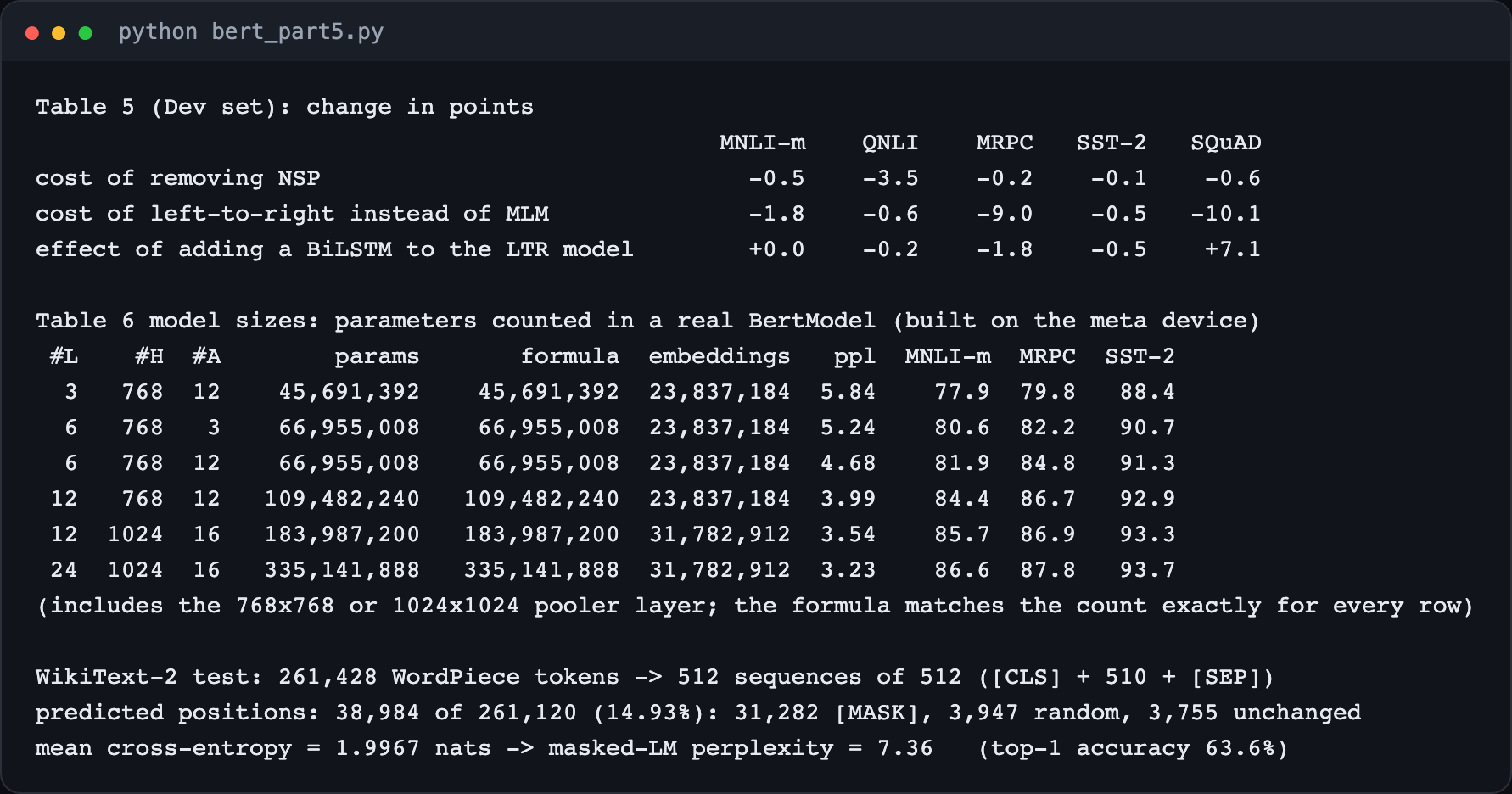
Numbers in a table are easier to compare as differences. My script bert_part5.py subtracts each row from the row before (the Table 5 values are typed in from the paper):

Table 5 (Dev set): change in points
                                                MNLI-m    QNLI    MRPC   SST-2   SQuAD
cost of removing NSP                              -0.5    -3.5    -0.2    -0.1    -0.6
cost of left-to-right instead of MLM              -1.8    -0.6    -9.0    -0.5   -10.1
effect of adding a BiLSTM to the LTR model        +0.0    -0.2    -1.8    -0.5    +7.1

Row 1 to row 2: removing NSP.

Looking at the computed differences, the NSP claim is weaker than the word "significantly" suggests. QNLI really drops (3.5 points), but MNLI drops 0.5 and SQuAD 0.6, and MRPC and SST-2 barely move (0.2 and 0.1). The paper does not report how much these Dev scores vary between runs, so we cannot tell how much of a 0.5-point gap is noise. Keep this in mind: in Part 6 we will see that later work (RoBERTa) questioned whether NSP is needed at all.

Row 2 to row 3: one direction instead of two. This is the big one. With everything else equal, going from the masked LM to a left-to-right LM costs 9.0 points on MRPC and 10.1 points of F1 on SQuAD, and loses something on every task. This is the cleanest evidence in the paper that the bidirectional design, not just more data or a bigger batch, explains much of BERT's gain.

Why does SQuAD suffer most? SQuAD needs a start and an end position for the answer (Part 4). Whether a word is the end of an answer depends heavily on the words after it. In an LTR model, the vector for each token was built without ever seeing those words. The BiLSTM adds right-side context, which is why SQuAD jumps by 7.1 points (77.8 to 84.9). But it is one small layer trained only on the task data, while BERT mixes both sides in all 12 layers during pre-training. The result is still 3.6 points below BERT-base (84.9 versus 88.5).

On the GLUE tasks the BiLSTM does not help at all (MNLI unchanged, the others down by 0.2 to 1.8 points). A plausible reason, not tested in the paper: a randomly initialized layer has to be learned from small task datasets, and MRPC has only a few thousand training pairs (3,600, according to Section 5.2).

Why not just do what ELMo does?#

Each argument in plain words:

• (a) Cost. Two full models to pre-train and to run, instead of one.
• (b) Question answering. In BERT's input the question comes first and the paragraph second (Part 4). A right-to-left model reading the paragraph has not reached the question yet (the question is to its left), so its vectors for the paragraph words know nothing about what is being asked.
• (c) Depth. In ELMo the two directions meet only at the very end. In BERT, every layer mixes both sides, so later layers can build on information that already combines left and right. A small grammar slip in the paper can confuse readers here: in "this it is strictly less powerful ... since it can use both left and right context at every layer", the second "it" means the deep bidirectional model, not the concatenation.

Argument (a) is easy to measure. I built an LTR stack and an RTL stack of BERT-base size and timed them against one bidirectional model (bert_part5_math.py):

parameters: one bidirectional model 109,482,240; LTR + RTL = 218,964,480
vector per token: bidirectional (512, 768) ; LTR (512, 768) + RTL (512, 768) -> concat (512, 1536)
time for a batch of 8 x 512 tokens on mps (median of 5): one model 133 ms, LTR + RTL 261 ms -> 1.96x
in a sequence of 6 tokens, which positions can token 3 use (1-based)?
  bidirectional, any layer: [1, 2, 3, 4, 5, 6]
  LTR stack, any layer:     [1, 2, 3]    RTL stack, any layer: [3, 4, 5, 6]
  concatenation: both lists, but only side by side at the very top; no layer ever mixes them

Twice the parameters and 1.96 times the time, as the paper says. And the last lines are argument (c) in miniature: in the glued model, no single layer ever combines token 1 with token 6 when building token 3.

How ELMo actually combines its layers, in its own paper:

where $h_{k,j}$ is the (forward and backward, concatenated) vector of token $k$ at layer $j$, and the task model learns the $L + 1$ weights $s_j$ and the single number $\gamma$; the LSTMs themselves stay frozen.

The other differences between BERT and GPT#

Table 5's LTR & No NSP row matters for one more reason, which the paper explains in Appendix A.4.

The logic: the LTR & No NSP model is GPT's recipe (left to right, no NSP) but trained with all four of BERT's advantages (BERT's data, BERT's input format, BERT's batch size, BERT's fine-tuning). So any gap between LTR & No NSP and BERT-base cannot come from those four things. It must come from the masked LM, which gives bidirectionality, and NSP. And that gap is large: up to 9.2 points on MRPC (77.5 versus 86.7) and 10.7 on SQuAD (77.8 versus 88.5).

Effect of model size#

A small inconsistency: the text says "all four datasets", but Table 6 shows three tasks (MNLI-m, MRPC, SST-2). The paper does not say what the fourth one is.

You met L, H and A in Part 2. The new column is perplexity.

For a masked LM, the perplexity is computed over the positions the model has to predict:

where:

• $N$ is the number of predicted (masked) positions;
• $x_i$ is the true token at the $i$-th predicted position;
• $p(x_i \mid \text{context})$ is the probability the model gave to that true token, from its softmax over the vocabulary;
• $\log$ is the natural logarithm, and the minus sign makes the sum positive: the inside of the bracket is the average cross-entropy loss (Part 3);
• $\exp$ ("e to the power of") undoes the logarithm, turning an average loss into a number of "equally likely choices".

So BERT-base's 3.99 means: on its held-out training text, when it predicts a masked token, it is on average about as unsure as a choice between 4 words.

How many parameters is each row?#

Where the per-layer term $12H^2 + 13H$ comes from, piece by piece (all for one layer with hidden size $H$ and feed-forward size $4H$):

For $H = 768$: $12 \times 768^2 + 13 \times 768 = 7{,}077{,}888 + 9{,}984 = 7{,}087{,}872$ parameters per layer.

The paper gives parameter counts only for BERT-base and BERT-large. I built every model of Table 6 with the Hugging Face BertConfig (30,522-token vocabulary, 512 positions, feed-forward size 4H, as in Part 2) on PyTorch's meta device, which creates the shapes without allocating any memory, and counted:

import torch
from transformers import BertConfig, BertModel

for L, H, A in [(3, 768, 12), (6, 768, 3), (6, 768, 12), (12, 768, 12), (12, 1024, 16), (24, 1024, 16)]:
    cfg = BertConfig(vocab_size=30522, hidden_size=H, num_hidden_layers=L, num_attention_heads=A,
                     intermediate_size=4 * H, max_position_embeddings=512, type_vocab_size=2)
    with torch.device("meta"):              # shapes only, no memory
        model = BertModel(cfg)
    print(L, H, A, sum(p.numel() for p in model.parameters()))

 #L    #H  #A        params       formula  embeddings   ppl  MNLI-m  MRPC  SST-2
  3   768  12    45,691,392    45,691,392  23,837,184  5.84    77.9  79.8   88.4
  6   768   3    66,955,008    66,955,008  23,837,184  5.24    80.6  82.2   90.7
  6   768  12    66,955,008    66,955,008  23,837,184  4.68    81.9  84.8   91.3
 12   768  12   109,482,240   109,482,240  23,837,184  3.99    84.4  86.7   92.9
 12  1024  16   183,987,200   183,987,200  31,782,912  3.54    85.7  86.9   93.3
 24  1024  16   335,141,888   335,141,888  31,782,912  3.23    86.6  87.8   93.7

The "formula" column is the count from the equation of Part 2 (embeddings, plus $12H^2 + 13H$ per layer, plus the $H \times H$ pooler), and it matches the real model exactly in every row. Three things stand out:

• BERT-base is 109.5M and BERT-large is 335.1M parameters, counted this way. The paper rounds them to "110M" and "340M". (Part 2 discusses the 340M.)
• The two 6-layer models have exactly the same number of parameters (66,955,008), yet 12 heads beat 3 heads on all three tasks (MNLI-m 81.9 versus 80.6). The number of heads only changes how the same $H \times H$ matrices are split up, not how many numbers they hold.
• The embeddings are a big share of small models. In the 3-layer model, 23.8M of its 45.7M parameters (52%) are embeddings, the word-lookup table alone.

Was this big for 2018?#

The two comparison models, in their own papers:

Can we check these two numbers with our formula? Only roughly, because both models differ from BERT in their embeddings and outputs:

Vaswani et al. 2017, big encoder: L=6, H=1024: the layers alone, if shaped like BERT's (12H^2 + 13H each) = 75,577,344   (paper says 100M for the encoder)
Al-Rfou et al. 2018: L=64, H=512: the layers alone, if shaped like BERT's (12H^2 + 13H each) = 201,752,576   (paper says 235M)

The layers alone give 75.6M and 201.8M. The rest of the published totals is embeddings and other parts (the big Transformer's shared vocabulary table of about 37,000 tokens × 1,024 adds roughly 38M). So the orders of magnitude agree; the exact numbers depend on details these papers do not spell out in the same way.

Note the careful word "hypothesize": the paper offers an explanation for why fine-tuning scales where feature-based approaches did not, but does not test it directly. The measured fact is Table 6 itself.

A real perplexity, for scale#

First, the definition with a toy you can follow. For $N$ predicted words with probabilities $p_1, \dots, p_N$ given to the true words:

where NLL is the mean negative log-likelihood in nats (natural-log units). Sanity check: a model that is uniform over 4 words gives every word $p = 1/4$, so NLL $= \log 4 = 1.386$ and perplexity $= 4$: "as unsure as a 4-way guess".

A real sentence, three masked words, bert-base-uncased:

input: she opened the [MASK] with her [MASK] and walked into the [MASK] .
door     p = 0.9586   -log p = 0.0423   (top 3 guesses: door, gate, box)
key      p = 0.1324   -log p = 2.0222   (top 3 guesses: key, hand, keys)
kitchen  p = 0.1823   -log p = 1.7022   (top 3 guesses: room, kitchen, house)
mean NLL = (0.0423 + 2.0222 + 1.7022) / 3 = 1.2554 nats -> perplexity = exp(1.2554) = 3.51
GPT-2 mean NLL = 3.7125 -> perplexity 40.96  (same three words, left context only)

BERT's 3.51 here is close to Table 6's numbers (3.23 to 5.84), but it is one sentence. (GPT-2's 40.96 is not a fair comparison: it predicts each word from the left side only, a harder task.)

What does a masked-LM perplexity of about 4 look like on real text? I measured the released bert-base-uncased on the test split of WikiText-2, a public set of Wikipedia articles, using the paper's masking recipe (15% of tokens chosen; of those 80% [MASK], 10% random, 10% unchanged), sequences of 512 tokens, and a fixed random seed:

chosen = torch.rand(x.shape) < 0.15                    # pick 15% of positions
chosen[:, 0] = chosen[:, -1] = False                   # never [CLS] or [SEP]
r = torch.rand(x.shape)
inp = x.clone()
inp[chosen & (r < 0.8)] = tok.mask_token_id            # 80%: [MASK]
rnd = chosen & (r >= 0.8) & (r < 0.9)                  # 10%: a random token
inp[rnd] = torch.randint(len(tok), x.shape)[rnd]       # the other 10% stay unchanged
logp = torch.log_softmax(model(input_ids=inp).logits[chosen], -1)
nll += -logp.gather(1, x[chosen][:, None]).sum()       # cross-entropy on the chosen positions only

WikiText-2 test: 261,428 WordPiece tokens -> 512 sequences of 512 ([CLS] + 510 + [SEP])
predicted positions: 38,984 of 261,120 (14.93%): 31,282 [MASK], 3,947 random, 3,755 unchanged
mean cross-entropy = 1.9967 nats -> masked-LM perplexity = 7.36   (top-1 accuracy 63.6%)

So on this text the released model has a perplexity of 7.36, and its first guess is right 63.6% of the time. That is higher (worse) than the 3.99 in Table 6. I cannot reproduce the paper's number, and the comparison is not like for like:

• The paper measured "held-out training data": text from the same BooksCorpus and Wikipedia mix BERT was trained on. WikiText-2 is a different sample, with its own formatting (I undid its @-@ style marks and dropped headings, but other differences remain).
• Table 6's models are the ablation models, trained with the same procedure; the paper does not say the 3.99 was measured on the released checkpoint.
• My random replacements draw from the whole vocabulary, including rarely used tokens.

What the measurement does show: the 15% / 80-10-10 recipe behaves as described (14.93% of positions chosen, split 80.2% / 10.1% / 9.6%), and a single-digit perplexity on unseen text is in the same range as Table 6's numbers.

Feature-based approach with BERT#

Part 1 introduced two ways to reuse a pre-trained model: feature-based (freeze it, use its vectors) and fine-tuning (train everything). Every BERT result so far was fine-tuned. Section 5.3 asks whether frozen BERT features are good too.

Use case. A team wants to try twenty different classifiers on a million documents. Fine-tuning means twenty full BERT training runs. Feature-based means running BERT once over the million documents, saving the vectors, and training twenty small models on the saved vectors, each in minutes.

The tags come from the CoNLL-2003 data format, described in its own paper:

Why would a CRF help? A per-token classifier picks each tag on its own, and can produce impossible sequences. A toy with hand-made scores for three words (rows) and three tags (columns):

scores (rows = words ['met', 'Ada', 'Lovelace'], columns = ['O', 'B-PER', 'I-PER']): 3.0, 0.5, 0.2; 1.2, 1.0, 0.4; 0.3, 0.6, 2.5
per-token argmax: ['O', 'O', 'I-PER']  (sum 6.7; O followed by I-PER is invalid)
best valid sequence: ['O', 'B-PER', 'I-PER']  (sum 6.5)

The six feature choices in Table 7 read different hidden states:

Reading Table 7 carefully:

• Fine-tuning: BERT-large 96.6 Dev / 92.8 Test, BERT-base 96.4 / 92.4. Note the word "competitively": on the Test set, CSE (93.1) is higher than BERT-large (92.8). NER is not one of BERT's eleven new records.
• Embeddings alone: 91.0. The embedding output is the word-lookup vector plus position and segment, before any attention. It knows nothing about the sentence. Context is worth more than 5 points here.
• Last hidden 94.9 is worse than second-to-last 95.6. One common explanation (not tested in the paper): the last layer is shaped most strongly by the pre-training tasks, predicting masked words, so the layer before it holds more general information.
• Combining layers helps: weighted sum of the last four 95.9, concatenating them 96.1. Summing all 12 layers (95.5) is worse than using only the top four.
• 96.1 versus 96.4: the best frozen choice is 0.3 points behind fine-tuned BERT-base on Dev.

The frozen-feature tagger of Section 5.3, shape by shape, on "Ada Lovelace met Charles Babbage in London .":

WordPiece tokens               [13]
all hidden states              [13, 13, 768]
first sub-token of each word   [8, 13, 768]
concat last four layers        [8, 3072]
BiLSTM output                  [8, 768]
tag scores                     [8, 9]
BiLSTM layer 1 (input 3072): 2 directions x 4 x (384*3072 + 384*384 + 2*384) = 10,622,976
BiLSTM layer 2 (input 768):  2 directions x 4 x (384*768 + 384*384 + 2*384)  = 3,545,088
classifier 9 x 768 + 9 = 6,921;  tagger total 14,174,985 trainable, BERT-base-cased frozen (108,310,272 parameters never change)

The LSTM count: each direction has 4 gates, each gate a matrix from the input (3,072 numbers) and one from its own previous state (384 numbers), plus two bias vectors in the PyTorch layout: $4 \times (384 \times 3072 + 384 \times 384 + 2 \times 384)$ per direction.

Can we see the same pattern ourselves? I ran a smaller version of the experiment in bert_part5_ner.py:

• Model: bert-base-cased, frozen (no weight of BERT changes).
• Data: CoNLL-2003 from the Hugging Face hub (eriktks/conll2003). Training: the first 5,000 of the 14,041 training sentences. Evaluation: the whole Dev set, 3,250 sentences (51,362 words). Each sentence is read on its own: this copy of the dataset has no document boundaries, so there is no "maximal document context".
• Features: all 13 hidden states, first sub-token of every word, saved once.
• Classifier: a 2-layer BiLSTM with 384 units per direction (768 in total, my reading of "768-dimensional"), then a linear layer over the 9 tags; Adam, learning rate 0.001, batch 32, 4 epochs. Each choice trained with 3 seeds, averaged (the paper used 5).
• Score: entity-level F1 on Dev, computed by my own code (an entity counts as correct only if its type and its exact span match).

The heart of the feature extraction:

enc = tok(words, is_split_into_words=True, return_tensors="pt")
with torch.no_grad():                                                  # BERT is frozen
    hs = torch.stack(bert(**enc, output_hidden_states=True).hidden_states, 2)[0]   # (tokens, 13, 768)
wid = enc.word_ids(0)                                                  # which word each token belongs to
first = [t for t, w in enumerate(wid) if w is not None and (t == 0 or wid[t - 1] != w)]
features = hs[first]                                                   # (words, 13, 768): first sub-token only

concat_last_four = features[:, 9:13].flatten(1)                        # (words, 3072)
weighted_last_four = (torch.softmax(w, 0)[None, :, None] * features[:, 9:13]).sum(1)   # w: 4 learned weights

The results:

CoNLL-2003: 5000 training sentences used, 3250 dev sentences; labels: ['O', 'B-PER', 'I-PER', 'B-ORG', 'I-ORG', 'B-LOC', 'I-LOC', 'B-MISC', 'I-MISC']
features: 67634 train words, 51362 dev words, 13 layers x 768 numbers each, 34 s
Embeddings                   dev F1 = 82.66   (seeds: 82.73, 82.42, 82.82; 113 s)
Second-to-last hidden        dev F1 = 89.94   (seeds: 88.72, 90.25, 90.84; 127 s)
Last hidden                  dev F1 = 88.64   (seeds: 88.13, 89.03, 88.77; 161 s)
Weighted sum last four       dev F1 = 90.37   (seeds: 90.08, 90.00, 91.05; 311 s)
Concat last four             dev F1 = 91.17   (seeds: 90.94, 91.41, 91.16; 484 s)
Weighted sum all 12 layers   dev F1 = 90.49   (seeds: 91.28, 89.60, 90.59; 450 s)

Lined up against Table 7:

What agrees with the paper:

• The embeddings alone are clearly worst (82.66), about 6 to 8.5 points below every choice that uses BERT's layers. Context is what BERT adds.
• Concatenating the last four layers is best (91.17), in both the paper and our run.
• The second-to-last layer beats the last layer (89.94 versus 88.64), as in the paper (95.6 versus 94.9).
• Combining the top four layers beats any single layer, whether summed or concatenated.

What does not agree: in our run the weighted sum of all 12 layers (90.49) edges out the weighted sum of the last four (90.37), the opposite of the paper's order. The gap is 0.12 points, while the three seeds of the 12-layer choice alone range from 89.60 to 91.28, so this run cannot separate those two.

Our absolute numbers are about 5 to 8.5 points lower than the paper's. That is expected, not a contradiction: we trained on 5,000 of the 14,041 sentences, for 4 epochs, with no hyperparameter search, and without the document context the paper adds to every sentence. We also did not fine-tune BERT, so this experiment says nothing about the 96.4 of fine-tuning; it only checks the shape of the feature-based rows.

How long to pre-train#

The last two ablations are in Appendix C. The first asks whether BERT's long pre-training is necessary.

The total pre-training in Question 1 is the paper's own product: 128,000 words per batch × 1,000,000 steps = 128 billion words processed (with the paper's rounding of 256 × 512 = 131,072 to 128,000, as in Part 3).

How to read it:

• Both curves rise, then flatten. More pre-training always helped, but with smaller gains later on.
• The MLM curve is still climbing between 500k and 1M steps: that is the "almost 1.0%" of Question 1.
• At the very first checkpoint the left-to-right model is ahead, which fits "converges slightly slower": it gets a training signal from every word, the MLM from only 15%. But the MLM curve passes it straight away and the gap then widens to about 2 points by the end (reading the figure, not a number printed in the paper).

The trade-off is worth it. The MLM sees fewer training signals per batch, but each one uses context from both sides.

How many predictions does each objective get from one batch?

one batch = 256 x 512 = 131,072 tokens; masked LM predicts 15% = 19,661; left-to-right LM predicts every next token, about 131,072
over 1,000,000 steps: 19,661,000,000 masked-LM predictions versus about 131,072,000,000 for LTR (6.67x more)

That is the "converges slightly slower" of Question 2, made concrete: per step the masked LM learns from 6.67 times fewer predictions. Figure 5 shows it is still the better choice.

Masking strategies#

Part 3 explained the 80/10/10 masking recipe and why the paper uses it. Appendix C.2 tests whether it was a good choice.

Why would the mismatch be worse for frozen features? With fine-tuning, every weight of BERT is adjusted on the task's real sentences, so the model can unlearn any habit tied to [MASK]. With frozen features, BERT is used exactly as pre-trained. If its vectors for ordinary, unmasked words are not very informative (because it was never asked to predict an unmasked word), nothing can fix that afterwards.

Row by row:

1. 80 / 10 / 10 (BERT's recipe): 84.2, 95.4, 94.9. The best NER scores in both columns.
2. 100 / 0 / 0 (always [MASK]): MNLI 84.3 is fine, but feature-based NER drops to 94.0, the worst value in that column and 0.9 below BERT's recipe. This is the predicted mismatch: the model only ever had to predict at [MASK], and its frozen vectors for normal words are less useful.
3. 80 / 0 / 20: 84.1, 95.2, 94.6. Random replacement without any "keep" cases.
4. 80 / 20 / 0: 84.4, 95.2, 94.7. Interestingly the best MNLI score in the table, 0.2 above BERT's recipe.
5. 0 / 20 / 80 (no [MASK] at all): 83.7, 94.8, 94.6.
6. 0 / 0 / 100 (always random): 83.6 on MNLI, the worst. Here the model is trained to find and fix wrong words, and 15% of every training input is noise.

Putting numbers on "robust": across all six recipes, MNLI moves within 0.8 points (83.6 to 84.4) and fine-tuned NER within 0.6 (94.8 to 95.4). Feature-based NER moves within 0.9 (94.0 to 94.9), with always-[MASK] at the bottom. These are small differences, single numbers without error bars, so the honest summary is: the masking recipe matters little when you fine-tune, and a bit more when you freeze.

One more detail, which the paper does not explain: BERT's own row here scores 84.2 on MNLI, while the BERT-base row of Table 5 scores 84.4. They are probably different training runs, but the paper does not say.

Next, in Part 6: what happened after BERT. Later work revisited exactly these ablations (RoBERTa dropped NSP; ALBERT, DistilBERT and ELECTRA changed size and the masked LM itself), BERT's limits, how it is used today, and a summary of the whole paper.

Run it yourself

The scripts behind every measured number in this part:

• code/papers/bert/bert_part5.py: the Table 5 differences, the Table 6 parameter counts, and the WikiText-2 perplexity. About 6 minutes on a laptop CPU.
• code/papers/bert/bert_part5_ner.py: the frozen-feature NER experiment. It took about 28 minutes on an Apple M5 Pro GPU that was shared with other jobs at the time.

bashCopy

pip install torch transformers datasets
python bert_part5.py        # writes results/part5.json
python bert_part5_ner.py    # writes results/part5_ner.json

References#

The BERT paper

1. J. Devlin, M.-W. Chang, K. Lee, K. Toutanova. BERT: Pre-training of Deep Bidirectional Transformers for Language Understanding. NAACL 2019 (ACL Anthology).
2. Google Research. BERT code and models, including extract_features.py and the cased models.

Papers the BERT paper cites in this part

3. A. Radford, K. Narasimhan, T. Salimans, I. Sutskever. Improving Language Understanding by Generative Pre-Training (OpenAI GPT). OpenAI, 2018.
4. M. E. Peters et al. Deep contextualized word representations (ELMo, "2018a"). NAACL 2018.
5. M. E. Peters, M. Neumann, L. Zettlemoyer, W. Yih. Dissecting Contextual Word Embeddings: Architecture and Representation ("2018b", the mixed results on bi-LM size). EMNLP 2018.
6. O. Melamud, J. Goldberger, I. Dagan. context2vec: Learning Generic Context Embedding with Bidirectional LSTM. CoNLL 2016.
7. A. Vaswani et al. Attention Is All You Need. NeurIPS 2017.
8. R. Al-Rfou, D. Choe, N. Constant, M. Guo, L. Jones. Character-Level Language Modeling with Deeper Self-Attention. AAAI 2019.
9. E. F. Tjong Kim Sang, F. De Meulder. Introduction to the CoNLL-2003 Shared Task: Language-Independent Named Entity Recognition. CoNLL 2003.
10. K. Clark, M.-T. Luong, C. D. Manning, Q. V. Le. Semi-Supervised Sequence Modeling with Cross-View Training (CVT, Table 7). EMNLP 2018.
11. A. Akbik, D. Blythe, R. Vollgraf. Contextual String Embeddings for Sequence Labeling (CSE, Table 7). COLING 2018.

Other sources used in this part

12. L. A. Ramshaw, M. P. Marcus. Text Chunking using Transformation-Based Learning (the IOB tagging scheme). Workshop on Very Large Corpora, 1995.
13. S. Merity, C. Xiong, J. Bradbury, R. Socher. Pointer Sentinel Mixture Models (WikiText-2). ICLR 2017.
14. Code for this part: bert_part5.py, bert_part5_ner.py, bert_part5_math.py.