BERT, explained · Part 1 of 6 · Covers Title, Abstract, §1

The Big Idea: Reading in Both Directions

The title, the abstract and the introduction of the BERT paper, line by line: what pre-training is, the two ways to reuse a pre-trained model, why reading only left to right is a real limit, and BERT's fix of filling in blanks. With a real run of GPT-2 and BERT on the same sentences.

BERT: Pre-training of Deep Bidirectional Transformers for Language Understanding. Jacob Devlin, Ming-Wei Chang, Kenton Lee, Kristina Toutanova. NAACL 2019, 2018. arXiv:1810.04805

In October 2018, four researchers at Google posted a paper called BERT. It reported new best results on eleven language tasks at once. A year later, in October 2019, Google wrote that BERT would help its search engine understand about one in ten English searches in the US. BERT-style models are still used today inside search engines, spam filters, support-ticket routers and retrieval systems.

This series reads the paper slowly, in the paper's own order. Each piece follows the same pattern:

1. The exact lines from the paper, as a highlighted screenshot in a teal box like the one below.
2. A plain-English explanation, with a yellow box for every new word.
3. A picture, and real code when it helps, with its real output.
4. Why it matters, and only then the next piece.

The small Paper §1 tag above each heading tells you which section of the paper you are reading. The screenshots come from the paper's second arXiv version (May 2019), the one most people read today.

The title#

Let us take the title apart, one word at a time.

• Pre-training. First, train a model on a huge pile of ordinary text, before it ever sees the real task. This is the expensive part, and it is done once.
• Deep. The model is a tall stack of layers (12 or 24 of them). Each layer refines what the layer below understood.
• Bidirectional. Every word looks at the words on its left and on its right. This is the key idea of the paper.
• Transformers. The kind of neural network used. It was introduced in 2017 in the paper Attention Is All You Need.
• Language Understanding. The goal: tasks where a model must understand text (classify it, answer questions about it, find names in it), not write new text.

What BERT is#

The name has four parts. You already know bidirectional and transformers from the title. The two new words are encoder and representations.

Encoder and decoder: the two halves of the Transformer#

"Encoder" is a precise word here. It points at one half of the Transformer from Attention Is All You Need (Vaswani et al., 2017), the paper BERT is built on.

That rule is implemented by a mask inside attention. Here is attention with the mask written in. (The attention series derives this equation step by step.)

where, for a text of $n$ tokens:

• $Q$, $K$, $V$ are the queries, keys and values: three $n \times d_k$ tables made from the token vectors. Row $i$ of $Q$ asks "what is token $i$ looking for?"; row $j$ of $K$ says "what does token $j$ offer?";
• $QK^\top$ is an $n \times n$ table of scores: entry $(i, j)$ says how well token $i$'s question matches token $j$;
• $\sqrt{d_k}$ (here $\sqrt{64} = 8$) keeps the scores from growing too large;
• $M$ is the mask, also $n \times n$: 0 where looking is allowed, $-\infty$ where it is blocked;
• softmax turns each row into weights that add up to 1, and $e^{-\infty} = 0$, so a blocked position gets weight exactly 0.

The two models differ only in $M$:

In words: GPT blocks every key to the right of the query (the upper triangle of the table). BERT blocks nothing. (BERT's real code also masks padding, the empty slots that fill short texts up to a common length, but never real words.)

A worked example with real numbers. I took the first attention head of GPT-2's first layer, fed it "the kid smiles", and recomputed the attention by hand (bert_part1_math.py):

q, k, v = blk.attn.c_attn(blk.ln_1(x)).split(768, dim=2)      # GPT-2 layer 1: queries, keys, values
qh, kh = q[0, :, 0:64], k[0, :, 0:64]                          # head 1 uses 64 of the 768 numbers
S = (qh @ kh.T) / math.sqrt(64)                                # 3 x 3 table of scores
M = torch.triu(torch.full((3, 3), float('-inf')), diagonal=1)  # -inf above the diagonal: the future
A = torch.softmax(S + M, -1)                                   # each row adds up to 1

scores s = q.k / sqrt(64):
  the     -0.618   -1.104   -0.860
  kid      0.770   -0.374   -0.562
  smiles   0.345   -0.316   -0.987
mask M (0 = allowed, -inf = blocked: a key to the right of the query):
  the      0.000     -inf     -inf
  kid      0.000    0.000     -inf
  smiles   0.000    0.000    0.000
weights a = softmax(s + M), row by row:
  the      1.000    0.000    0.000   (row sum 1.000)
  kid      0.758    0.242    0.000   (row sum 1.000)
  smiles   0.562    0.290    0.148   (row sum 1.000)
max difference from the library's own attention weights: 0.0e+00

Follow the row for "kid" by hand. Its score for "smiles" (-0.562) is replaced by $-\infty$, so only two scores are left:

The first row is even simpler: "the" can see only itself, so its weight on itself is 1.000 whatever its score is. Our hand computation matches the library exactly (difference 0.0).

So when the paper says BERT is "bidirectional", this is the concrete meaning: an all-zero mask. The hard part, which the rest of the paper solves, is how to train such a model, since the usual training game (predict the next word) breaks when the model can see the next word.

The abstract makes three claims. Let us translate each one.

1. "Pre-train deep bidirectional representations from unlabeled text." BERT learns from text that nobody has labelled: Wikipedia and a collection of books. Nobody had to mark which sentences are happy or sad. Labelled data is expensive. Plain text is almost free, and there is a lot of it.

How can a model learn anything from text that has no answers attached? The trick is to make the answers out of the text itself. Hide a piece of the text, and the hidden piece is the answer.

2. "Jointly conditioning on both left and right context in all layers." When BERT builds the representation of a word, it uses the words before it and the words after it, and it does this at every layer, not just at the end. "Conditioning on" simply means "using as input".

3. "Fine-tuned with just one additional output layer." After pre-training, you take BERT, put one small new layer on top, and keep training the whole thing a little on your task. The same pre-trained BERT can become a sentiment classifier, a question-answering system or a name finder.

Use case. A company that wants to sort support emails into "billing", "bug report" and "feature request" does not need to teach a model English. It starts from pre-trained BERT and fine-tunes it on a few thousand labelled emails.

Why an "understanding" model, when GPT-style models can write?#

A fair question today: chat models write fluent text, so why read a paper about a model that does not write? Because writing is only one job. Many everyday language jobs are about reading and deciding: is this review positive, which department should get this email, where are the names in this contract, which passage answers this question. Images have the same split: generating a new picture is one job, recognising what is in a photo is another, and most practical vision systems do the second.

For understanding jobs, a model that sees the whole input at once is a natural fit, and it can be small and fast. That is why BERT-style models still run inside many search, classification and retrieval systems (Part 6 shows where).

What exactly gets trained when you fine-tune?#

This is a common point of confusion, so it is worth stating carefully. The paper is explicit (we will see it in Section 3): "all of the parameters are fine-tuned". During fine-tuning, every one of BERT's roughly 110 million weights keeps learning, together with the small new output layer, which is the only part that starts from random numbers.

The idea itself came from computer vision, which the paper mentions in its related work (Section 2.3, Part 2): train a big network once on ImageNet, a large labelled photo collection, then reuse it for many smaller tasks. BERT brings that recipe to language, with one difference: its first stage needs no labels at all.

The results in the abstract#

Here are the four results from the abstract, in plain words:

A note on the wording "7.7% point absolute improvement": it means the score went up by 7.7 points (for example from 72.8 to 80.5), not by 7.7 percent of the old score. Part 4 goes through every one of these tasks and every table of results.

Pre-training already worked, for two kinds of tasks#

Now the introduction. Its first paragraph sets the scene.

The paper names four example tasks:

The two token-level examples in that paragraph deserve a closer look, because both come back in Part 4.

Two ways to reuse a pre-trained model#

Both approaches, the paper says, pre-train with a language model. That word is the key to the whole argument, so let us define it carefully.

A language model reads left to right and predicts each word from the words before it. Written as an equation, the probability of a whole sentence is built up one word at a time:

where:

• $w_1, \dots, w_n$ are the words of the sentence, in order, and $n$ is how many there are;
• $P(w_i \mid w_1, \dots, w_{i-1})$ is the probability of word $i$ given (that is what the bar $\mid$ means) all the words before it;
• $\prod$ means "multiply all of these together", for $i$ from 1 to $n$.

Look at what is on the right of the bar: only earlier words. That is what unidirectional means. The training signal is free (the next word is always in the text), which is why language models are such a good way to pre-train. But each word only ever learns from its left.

The chain rule with real numbers. Here is the equation applied to "The kid smiles at the dog." by GPT-2 (bert_part1_math.py). Each row is one factor of the product: the probability GPT-2 gave the real next word, seeing only the words on its left.

 i  word     given (left side only)     P(word | left)    log P
 1  The      (start)                          0.037700   -3.278
 2  kid      The                              0.000040  -10.114
 3  smiles   The kid                          0.000257   -8.268
 4  at       The kid smiles                   0.087426   -2.437
 5  the      The kid smiles at                0.150418   -1.894
 6  dog      The kid smiles at the            0.002395   -6.034
 7  .        The kid smiles at the dog        0.177917   -1.726
sum of log P = -33.752
P(sentence) = exp(-33.752) = 2.196e-15
average negative log-likelihood = 4.822  (perplexity exp of that = 124.2)

Three things to notice:

• Multiplying tiny numbers underflows, so in practice everyone adds logarithms instead: $\log \prod_i p_i = \sum_i \log p_i$. Here the seven logs add up to $-33.752$, and $e^{-33.752} = 2.2 \times 10^{-15}$, the same probability.
• Training a language model means making this sum as large as possible over billions of sentences. Written as a loss to make small, it is the negative log-likelihood:

where $\mathcal{L}$ is the loss (lower is better) and the other symbols are as above. For our sentence, $\mathcal{L} = 33.752$, or $4.822$ per word.

• "kid" got only 0.00004. After "The", thousands of words are possible, so no single one gets much probability. Every word is predicted from its left only; the model never got to use "smiles at the dog" to help with "kid".

The problem: reading in only one direction#

Why is one direction a problem? Because the meaning of a word often depends on what comes after it. Read this sentence and stop at the blank:

I went to the ____

You cannot know the missing word. Now read the whole sentence:

I went to the ____ to deposit my paycheck.

Now it is obviously "bank". The clue was on the right. A left-to-right model building the representation of that position has not seen "deposit my paycheck" yet, so it cannot use it.

Let us test it on real models#

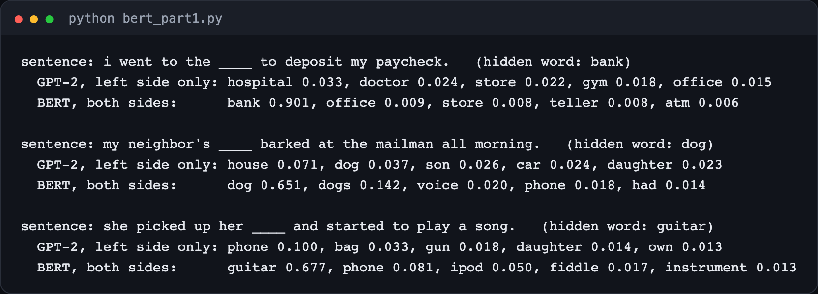
I gave the same three sentences to two real, public models:

• GPT-2, a left-to-right model from 2019 (the small version). It sees only the words before the blank and predicts the next word.
• BERT (bert-base-uncased, the model released with this paper). It sees the whole sentence with the blank replaced by a special [MASK] token, and predicts the missing word.

from transformers import AutoTokenizer, BertForMaskedLM, GPT2LMHeadModel
import torch

btok = AutoTokenizer.from_pretrained("bert-base-uncased")
bert = BertForMaskedLM.from_pretrained("bert-base-uncased").eval()
gtok = AutoTokenizer.from_pretrained("openai-community/gpt2")
gpt2 = GPT2LMHeadModel.from_pretrained("openai-community/gpt2").eval()

# GPT-2: only the left side, predict the next token
ids = gtok("I went to the", return_tensors="pt").input_ids
p_gpt2 = torch.softmax(gpt2(ids).logits[0, -1], -1)

# BERT: the whole sentence, predict the [MASK]
enc = btok("i went to the [MASK] to deposit my paycheck.", return_tensors="pt")
pos = (enc.input_ids[0] == btok.mask_token_id).nonzero().item()
p_bert = torch.softmax(bert(**enc).logits[0, pos], -1)

These are the five most likely words each model gave, with their probabilities (the real output of bert_part1.py):

sentence: i went to the ____ to deposit my paycheck.   (hidden word: bank)
  GPT-2, left side only: hospital 0.033, doctor 0.024, store 0.022, gym 0.018, office 0.015
  BERT, both sides:      bank 0.901, office 0.009, store 0.008, teller 0.008, atm 0.006

sentence: my neighbor's ____ barked at the mailman all morning.   (hidden word: dog)
  GPT-2, left side only: house 0.071, dog 0.037, son 0.026, car 0.024, daughter 0.023
  BERT, both sides:      dog 0.651, dogs 0.142, voice 0.020, phone 0.018, had 0.014

sentence: she picked up her ____ and started to play a song.   (hidden word: guitar)
  GPT-2, left side only: phone 0.100, bag 0.033, gun 0.018, daughter 0.014, own 0.013
  BERT, both sides:      guitar 0.677, phone 0.081, ipod 0.050, fiddle 0.017, instrument 0.013

Both sides do not make every word easy, though. Take "smiles" from our chain-rule sentence:

GPT-2  P(smiles | "The kid")                    = 0.0003   top 5: who 0.1939, is 0.0687, in 0.0596, was 0.0550, 's 0.0507
BERT   P(smiles | "the kid [MASK] at the dog.") = 0.0008   top 5: looked 0.3233, stared 0.1029, glanced 0.0795, pointed 0.0620, glared 0.0595

BERT's probability for "smiles" is still small, because "looked at the dog" fits just as well. But look at the kind of guesses. With only the left side, GPT-2's guesses are almost generic. With both sides, every one of BERT's top five is a verb that can be followed by "at". The right side did not reveal the answer; it narrowed the space of sensible answers. That narrowing is what makes BERT's vectors useful for understanding tasks.

What this shows, and what it does not:

• With the right side hidden, the guess is a guess. GPT-2's top answer for the first sentence has a probability of only 0.033.
• With both sides visible, the answer is nearly certain: BERT gives "bank" 0.901 and "guitar" 0.677.
• This is not a contest between two models. GPT-2 was simply not given the words on the right, because a left-to-right model never gets them at this position. That missing information is exactly the paper's point.

Use case. Question answering is the paper's own example. In "Who founded the company that makes the iPhone?", the word "company" needs the words after it to know which company. A model that builds every word's meaning from both sides can answer such questions far better.

BERT's fix: fill in the blanks#

If language models are one-directional by nature, how do you pre-train a two-directional model? The paper's answer is in the next paragraph.

You already saw masked language modelling in action: the [MASK] sentences above are exactly this pre-training task. The trick works because a hidden word cannot leak its own answer, so the model is free to look in both directions. In Part 3 we will see why an ordinary language model cannot simply look both ways (each word would "see itself"), and we will run the exact masking recipe, which has a few surprising details.

The paragraph ends with a second task, next sentence prediction: given two pieces of text, guess whether the second really came right after the first. Many tasks are about pairs of sentences (does this answer this question? does this sentence follow from that one?), and plain language modelling never practises that. Part 3 covers it too.

The three contributions#

Let us unpack each contribution.

1. Deep, not shallow, bidirectionality. ELMo does look both ways, but in a shallow way: one network reads left to right, another reads right to left, and their outputs are glued together ("concatenated") at the very end. Inside each network, information still flows one way only. In BERT, every layer of one single network mixes both sides. The paper argues this is "strictly more powerful".

To see what "shallow" means exactly, look at how ELMo is trained, in its own paper:

ELMo's objective, in the notation we used for GPT:

where $t_1, \dots, t_N$ are the tokens, the first term is the forward model (left side only) and the second the backward model (right side only). Each term on its own is an ordinary one-directional language model. No single term ever conditions on both sides at once, which is the thing BERT's masked language model does (Part 3).

2. Less hand-made machinery. Before BERT, the best question-answering systems and the best sentiment classifiers were different, carefully designed networks. With BERT, the same model plus one small output layer does both. That saves months of engineering per task.

3. Eleven state-of-the-art results, plus public code and weights. The public release is a big reason BERT spread so fast: anyone could download the model and fine-tune it on a single GPU. The model we ran above is that release.

Who's who: the papers BERT is talking to#

The introduction names a handful of earlier works again and again. Here they are in one place, so the rest of the series can refer back to them. Each entry is listed in full in the references at the end of this part.

GPT-2 (Radford et al., 2019, Language Models are Unsupervised Multitask Learners), which we ran above, came out a few months after BERT and is not cited in the paper. We use it only because it is a freely available left-to-right model of similar size.

Figure 3: the three designs side by side#

The paper puts its clearest picture of this argument in the appendix (Appendix A.4), so we read it now, where it belongs in the story.

How to read the figure:

• E₁, E₂, …, E_N (yellow, bottom) are the input embeddings: one vector per input token.
• Trm is one Transformer block (a layer). Lstm is one step of an LSTM, an older kind of network that reads one token at a time.
• T₁, T₂, …, T_N (green, top) are the output vectors, one per token.
• The arrows show who can see whom. In the BERT panel, every Trm connects to every position in the layer below. In the GPT panel, each Trm connects only to positions on its own left. In the ELMo panel, the arrows inside each LSTM chain all point one way; the two directions only meet at the top.

Notice also that BERT and GPT have the same shape: a stack of Transformer blocks. The only difference is the arrows, that is, which positions each token may look at. This is deliberate. The authors made BERT's smaller version the same size as GPT so the two could be compared fairly. Part 2 opens up that stack.

Next, in Part 2: the related work the paper builds on, and the model itself: its layers, its size (and where "110 million parameters" comes from), and how text becomes the numbers BERT reads.

Run it yourself

The script behind the GPT-2 and BERT comparison is code/papers/bert/bert_part1.py. It runs on a laptop CPU in under a minute and downloads bert-base-uncased (about 440 MB) and GPT-2 (about 550 MB) the first time.

bashCopy

pip install torch transformers
python bert_part1.py      # prints the table above, writes results/part1.json

References#

The BERT paper

1. J. Devlin, M.-W. Chang, K. Lee, K. Toutanova. BERT: Pre-training of Deep Bidirectional Transformers for Language Understanding. NAACL 2019 (ACL Anthology). arXiv:1810.04805, version 2 (May 2019), which is the version shown in the screenshots.
2. Google Research. BERT code and pre-trained models. GitHub, 2018.

Papers the BERT paper cites in this part

3. A. Vaswani, N. Shazeer, N. Parmar, J. Uszkoreit, L. Jones, A. N. Gomez, Ł. Kaiser, I. Polosukhin. Attention Is All You Need. NeurIPS 2017.
4. M. E. Peters, M. Neumann, M. Iyyer, M. Gardner, C. Clark, K. Lee, L. Zettlemoyer. Deep contextualized word representations (ELMo; "Peters et al., 2018a" in the paper). NAACL 2018.
5. A. Radford, K. Narasimhan, T. Salimans, I. Sutskever. Improving Language Understanding by Generative Pre-Training (OpenAI GPT). OpenAI technical report, 2018. The BERT paper's reference list gives it the title "Improving language understanding with unsupervised learning".
6. J. Howard, S. Ruder. Universal Language Model Fine-tuning for Text Classification (ULMFiT). ACL 2018.
7. A. M. Dai, Q. V. Le. Semi-supervised Sequence Learning. NeurIPS 2015.
8. W. L. Taylor. "Cloze Procedure": A New Tool for Measuring Readability. Journalism Quarterly 30(4), 1953 (cited as "Journalism Bulletin" in the BERT paper).
9. T. Mikolov, I. Sutskever, K. Chen, G. Corrado, J. Dean. Distributed Representations of Words and Phrases and their Compositionality (word2vec). NeurIPS 2013.
10. J. Pennington, R. Socher, C. D. Manning. GloVe: Global Vectors for Word Representation. EMNLP 2014.
11. R. Kiros, Y. Zhu, R. Salakhutdinov, R. Zemel, A. Torralba, R. Urtasun, S. Fidler. Skip-Thought Vectors. NeurIPS 2015.
12. B. McCann, J. Bradbury, C. Xiong, R. Socher. Learned in Translation: Contextualized Word Vectors (CoVe). NeurIPS 2017.
13. J. Deng, W. Dong, R. Socher, L.-J. Li, K. Li, L. Fei-Fei. ImageNet: A Large-Scale Hierarchical Image Database. CVPR 2009.

Other sources used in this part

14. A. Radford, J. Wu, R. Child, D. Luan, D. Amodei, I. Sutskever. Language Models are Unsupervised Multitask Learners (GPT-2). OpenAI, 2019. The openai-community/gpt2 model used in the code.
15. P. Nayak. Understanding searches better than ever before. Google blog, 25 October 2019.
16. Code for this part: bert_part1.py and bert_part1_math.py.