BERT, explained · Part 4 of 6 · Covers §3.2, §4, A.3, A.5, B.1

Fine-tuning and Results: GLUE, SQuAD and SWAG

Sections 3.2 and 4 of the BERT paper, line by line: how one pre-trained model becomes a classifier, a question answerer and a multiple-choice solver by adding a tiny output layer, and what the results tables really say. With a real fine-tune of BERT-base on SST-2 and MRPC, and our own span search scored on the full SQuAD dev sets.

BERT: Pre-training of Deep Bidirectional Transformers for Language Understanding. Jacob Devlin, Ming-Wei Chang, Kenton Lee, Kristina Toutanova. NAACL 2019, 2018. arXiv:1810.04805

Part 3 built a pre-trained BERT: a model that has read 3.3 billion words and learned to fill in blanks and to tell whether two sentences belong together. Nobody has asked it to do anything useful yet.

This part is about the second step of the recipe: fine-tuning. We read Section 3.2 (how fine-tuning works), then Section 4 (the experiments on eleven tasks), and the appendix sections that go with them (A.3, A.5 and B.1). Along the way we fine-tune BERT ourselves on a laptop GPU and check every formula in code.

One model, many tasks#

The key sentence is the last one. Put a question and a passage into one sequence, [CLS] question [SEP] passage [SEP], and let every token attend to every other token. A question word can now look at passage words, and a passage word can look at question words, in all 12 layers. That is cross attention, in both directions, for free. BERT needs no special pair-matching layer.

Plugging a task into BERT#

The output side has only two cases:

• Sentence-level tasks (one answer per input, like "positive" or "entailment") read the final vector of [CLS], called $C$, and add one small classification layer.
• Token-level tasks (one answer per token, like named-entity tags or the start and end of an answer) read the final vector of every token, $T_1, T_2, \dots$, and add one small layer that is applied to each token.

Why packing two texts into one sequence is enough#

Section 3.2 also makes a claim that is easy to read past: "encoding a concatenated text pair with self-attention effectively includes bidirectional cross attention between two sentences". Before BERT, models for text pairs encoded each text on its own, then added a special layer to compare them. The paper names two such systems:

It is not just a picture. In a public BERT-base fine-tuned for SQuAD, given "Where was Ada born?" and "Ada Lovelace was born in London in 1815.", question words really do look at the passage, in every layer (bert_part4_math.py):

layer  1: question -> passage 0.190   passage -> question 0.107   question -> [CLS]/[SEP] 0.306
layer  6: question -> passage 0.170   passage -> question 0.072   question -> [CLS]/[SEP] 0.503
layer 10: question -> passage 0.191   passage -> question 0.196   question -> [CLS]/[SEP] 0.414
layer 12: question -> passage 0.087   passage -> question 0.045   question -> [CLS]/[SEP] 0.740
averaged over all 12 layers and heads, "born" (question) gives 0.162 of its attention to the passage

(Each number is the average share of attention, over all heads, that flows from one block to the other. Much of the rest goes to [CLS] and [SEP], which many heads use as a resting place.)

Figure 4: the four shapes of a task#

The paper draws these cases in Appendix A.5.

How to read each panel:

• (a) Sentence pair classification. Two sentences go in; the red arrow comes out of $C$ only. Tasks: MNLI, QQP, QNLI, STS-B, MRPC, RTE, and SWAG.
• (b) Single sentence classification. One sentence; the arrow comes out of $C$. Tasks: SST-2, CoLA.
• (c) Question answering. Question and paragraph; the arrows come out of the paragraph tokens, marking where the answer starts and ends. Task: SQuAD v1.1.
• (d) Single sentence tagging. One sentence; an arrow comes out of every token with a tag such as B-PER (beginning of a person's name) or O (outside any name). Task: CoNLL-2003 NER, which Part 5 covers.

Fine-tuning is cheap#

We will test the "few hours on a GPU" claim ourselves later in this part, on a laptop.

The fine-tuning settings#

Which settings did the authors use for fine-tuning? Appendix A.3 answers.

The learning rates are tiny compared with pre-training (1e-4, Part 3). That is on purpose: the pre-trained weights are already good, and fine-tuning should nudge them, not overwrite them.

The size of the grid is 2 batch sizes × 3 learning rates × 3 epoch counts = 18 runs per task. With runs that take minutes, that is affordable.

Section 4: the experiments#

The nine GLUE tasks#

First, the benchmark's own summary table:

Before the results, let us meet the tasks. Appendix B.1 describes each one.

Here are all nine in plain words, with one made-up example each:

The classification layer#

The paper writes the loss in one breath. Let us write it out, for one example whose correct label is $y$:

where:

• $C$ is the final vector of the [CLS] token, a row of $H = 768$ numbers (for BERT-base);
• $W$ is the new weight matrix with $K$ rows (one per label) and $H$ columns, and $W^\top$ is it flipped, so $C\,W^\top$ gives one number per label;
• $\text{logits}_k$ is the score of label $k$, the dot product of $C$ with row $k$ of $W$;
• the fraction is the softmax, which turns the $K$ scores into probabilities that add up to 1;
• $y$ is the correct label, and the loss is minus the log of its probability.

The paper's "$\log(\text{softmax}(CW^T))$" is the log-probability of the right label; training maximises it, which is the same as minimising the loss above. (Real implementations also add a bias of $K$ numbers to the logits; the paper leaves it out of the formula.)

A toy example you can check by hand, with $H = 4$ and $K = 3$:

Each logit is the dot product of $C$ with one row of $W$:

Softmax: $e^{1.50} = 4.482$, $e^{-1.80} = 0.165$, $e^{-0.65} = 0.522$, which add up to $5.169$. So $P = (0.867,\ 0.032,\ 0.101)$, and if the right label is 0 the loss is $-\log 0.867 = 0.143$.

The same arithmetic on a real fine-tuned model, a public BERT-base fine-tuned on SST-2 (textattack/bert-base-uncased-SST-2), where label 1 means positive:

"a gorgeous, witty, seductive movie."  gold label 1
  C W^T = [-4.316, 4.135]  (library: [-4.316, 4.135])
  softmax = [0.0002, 0.9998];  loss = -log P(gold) = 0.0002
"the plot is dull and the acting is worse."  gold label 0
  C W^T = [3.883, -3.500]  (library: [3.883, -3.499])
  softmax = [0.9994, 0.0006];  loss = -log P(gold) = 0.0006

After fine-tuning, the gap between the two logits is large (8.45 and 7.38), so the model is very sure, and right, on both.

Checking the formula in code#

How many new weights is that? For a 3-label task, $W$ has $3 \times 768 = 2{,}304$ numbers, plus 3 for the bias: 2,307. I built the classifier by hand and compared it with the Hugging Face BertForSequenceClassification on the same weights:

from transformers import AutoTokenizer, BertForSequenceClassification
import torch

tok = AutoTokenizer.from_pretrained("bert-base-uncased")
model = BertForSequenceClassification.from_pretrained("bert-base-uncased", num_labels=3).eval()
enc = tok("A man is playing a guitar.", "A person is making music.", return_tensors="pt")
label = torch.tensor([0])

out = model(**enc, labels=label, output_hidden_states=True)
C = out.hidden_states[-1][:, 0]                       # final vector of [CLS], shape (1, 768)
pooled = torch.tanh(model.bert.pooler.dense(C))       # the "pooler" (see below)
W, b = model.classifier.weight, model.classifier.bias # W: (3, 768)
logits = pooled @ W.T + b                             # C W^T (+ bias)
loss = -torch.log_softmax(logits, -1)[0, label]       # -log softmax(C W^T)[y]

The real output (from bert_part4_heads.py):

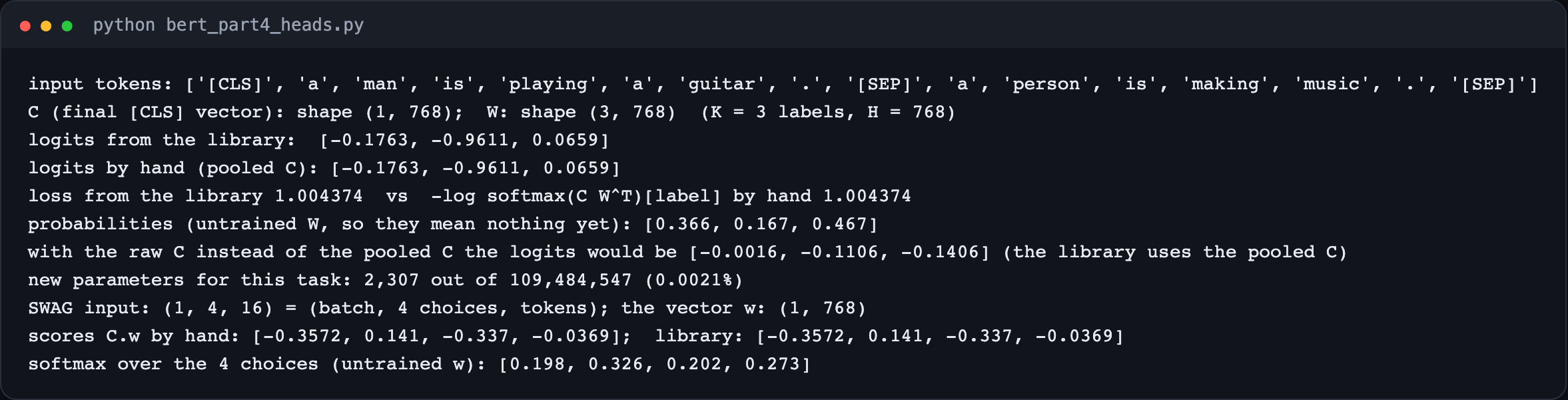
input tokens: ['[CLS]', 'a', 'man', 'is', 'playing', 'a', 'guitar', '.', '[SEP]', 'a', 'person', 'is', 'making', 'music', '.', '[SEP]']
C (final [CLS] vector): shape (1, 768);  W: shape (3, 768)  (K = 3 labels, H = 768)
logits from the library:  [-0.1763, -0.9611, 0.0659]
logits by hand (pooled C): [-0.1763, -0.9611, 0.0659]
loss from the library 1.004374  vs  -log softmax(C W^T)[label] by hand 1.004374
probabilities (untrained W, so they mean nothing yet): [0.366, 0.167, 0.467]
with the raw C instead of the pooled C the logits would be [-0.0016, -0.1106, -0.1406] (the library uses the pooled C)
new parameters for this task: 2,307 out of 109,484,547 (0.0021%)

The hand-written loss and the library's loss agree to all six printed decimals. The probabilities are meaningless here, because $W$ is still random: fine-tuning has not started.

Table 1: the GLUE results#

How to read it, column by column:

• The small numbers under the names are training-set sizes: MNLI has 392k examples, RTE only 2.5k. Keep these in mind: they explain where the biggest gains are.
• MNLI-(m/mm) has two numbers: accuracy on the "matched" test set (the same genres of text as the training data) and the "mismatched" set (different genres). BERT-large: 86.7/85.9.
• QQP, MRPC: F1 scores. STS-B: Spearman correlation. The rest: accuracy.
• Average: the plain average of the columns, which the caption says is "slightly different than the official GLUE score" because WNLI is left out.

And the rows:

• Pre-OpenAI SOTA: the best published result on each task before OpenAI GPT, each from a different specialised system.
• BiLSTM+ELMo+Attn: the GLUE paper's own baseline, a recurrent network using ELMo features.
• OpenAI GPT: the left-to-right Transformer from Part 1, fine-tuned the same way.
• BERT-base and BERT-large: one model each, one task at a time ("single-model, single task").

The two averages check out against the table: $79.6 - 75.1 = 4.5$ and $82.1 - 75.1 = 7.0$, where 75.1 is OpenAI GPT's average (the best earlier row). Note these are points, though the paper writes "%".

Two more sentences in this paragraph matter. First, "BERT-base and OpenAI GPT are nearly identical in terms of model architecture apart from the attention masking": the 4.5-point gap comes mostly from reading in both directions and from the pre-training tasks (Part 5 tests this). Second, footnote 9 says the GLUE test labels are hidden, and the authors "only made a single GLUE evaluation server submission for each of BERT-base and BERT-large". They did not tune on the test set.

Our own fine-tune: SST-2 and MRPC on a laptop GPU#

Reading a results table is one thing. Let us run the recipe. I fine-tuned the released bert-base-uncased on two GLUE tasks with the paper's settings, on the GPU of an Apple M5 Pro laptop:

• SST-2 (sentiment, 67,349 training sentences, 872 dev sentences);
• MRPC (paraphrase, 3,668 training pairs, 408 dev pairs).

The settings: batch size 32, 3 epochs, learning rate 2e-5 for SST-2 (one value from the paper's grid; I did not search), Adam with weight decay 0.01, the learning rate rising linearly over the first 10% of steps and then falling linearly to zero (as in Google's released run_classifier.py), dropout 0.1, one fixed seed. The classifier reads the pooled [CLS] vector, like the released code.

model = BertForSequenceClassification.from_pretrained("bert-base-uncased", num_labels=2).to("mps")
opt = torch.optim.AdamW(groups, lr=2e-5, weight_decay=0.01)   # no decay on biases and LayerNorm
steps = 3 * math.ceil(len(train) / 32)                         # 3 epochs, batch 32
warm = int(0.1 * steps)                                        # 10% warmup, then linear decay
sched = LambdaLR(opt, lambda s: s / warm if s < warm else (steps - s) / (steps - warm))

for ids, tt, am, y in batches(train):                          # every weight is trained
    loss = model(input_ids=ids, token_type_ids=tt, attention_mask=am, labels=y).loss
    loss.backward(); clip_grad_norm_(model.parameters(), 1.0)
    opt.step(); sched.step(); opt.zero_grad()

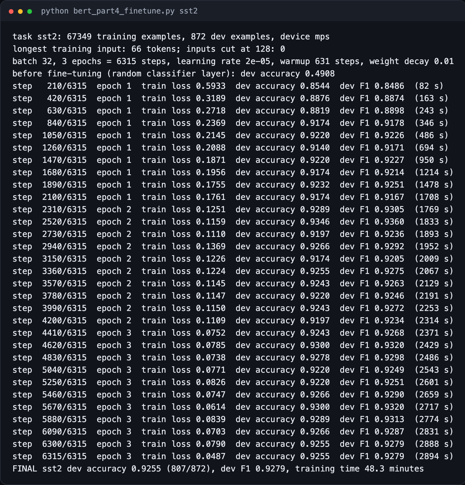
Here is the SST-2 run, the first and last lines of the real log (bert_part4_finetune.py):

task sst2: 67349 training examples, 872 dev examples, device mps
longest training input: 66 tokens; inputs cut at 128: 0
batch 32, 3 epochs = 6315 steps, learning rate 2e-05, warmup 631 steps, weight decay 0.01
before fine-tuning (random classifier layer): dev accuracy 0.4908
step   210/6315  epoch 1  train loss 0.5933  dev accuracy 0.8544  dev F1 0.8486  (82 s)
...
step  6300/6315  epoch 3  train loss 0.0790  dev accuracy 0.9255  dev F1 0.9279  (2888 s)
step  6315/6315  epoch 3  train loss 0.0487  dev accuracy 0.9255  dev F1 0.9279  (2894 s)
FINAL sst2 dev accuracy 0.9255 (807/872), dev F1 0.9279, training time 48.3 minutes

SST-2: 92.55% dev accuracy (807 of 872 sentences right), after 6,315 steps. Before fine-tuning, with a random $W$, the same model scored 49.1%: a coin flip. The paper reports 92.7 for BERT-base on the SST-2 dev set (Table 5, in Part 5) and 93.5 on the hidden test set (Table 1). Our single run, with one learning rate and no search, lands at 92.55. (During training, dev accuracy touched 93.5% at step 2,520; I report the model at the end of the 3 epochs, which is what a fixed number of epochs means, not the best checkpoint: picking the best checkpoint by its dev score would flatter the dev score.)

Note how fast it learns: dev accuracy was already 85.4% after the first 210 steps, which is about 10% of one epoch. Almost all of the knowledge was already in the pre-trained weights; fine-tuning only has to connect it to the two labels.

The run took 48 minutes of wall time on the laptop GPU, including 31 evaluations on the dev set, and other experiments were sharing the GPU for most of it, so treat the time as an upper bound. That matches the paper's "a few hours on a GPU" comfortably.

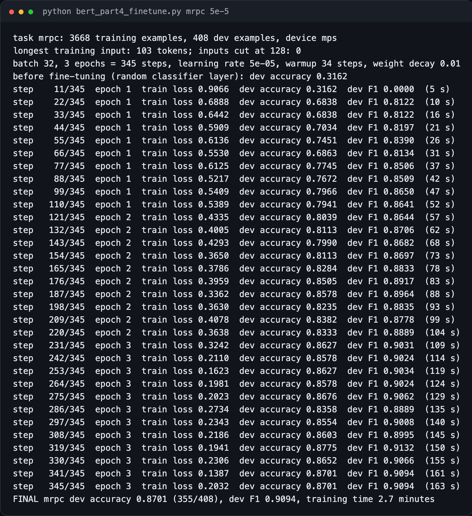
MRPC is the opposite kind of task: only 3,668 training pairs. Here I did what the paper did for GLUE and ran all four learning rates from its grid, one run each, keeping everything else fixed:

The best learning rate here is 5e-5, with 87.0% dev accuracy (355/408) and F1 90.9. The paper reports 86.7 dev accuracy for BERT-base on MRPC (Table 5). Three honest remarks:

• The same job is not even exactly repeatable. Before the grid, I had run the 2e-5 job once with the same seed and got 81.9% (334/408), against 83.3% in the grid. GPU arithmetic on the Apple GPU is not bit-for-bit repeatable, and on 408 dev examples one changed answer moves accuracy by 0.25 points. This is the instability the paper mentions, and why it reports "average Dev Set accuracy from 5 random restarts" in its model-size study (Part 5).
• The spread between learning rates is large for such a small dataset, which is exactly what Appendix A.3 warns about ("large data sets ... were far less sensitive to hyperparameter choice than small data sets").
• MRPC is lopsided: 68% of its pairs are paraphrases (the GLUE paper notes this), so always answering "yes" already scores about 68% on dev. Before fine-tuning, our random head answered "no" every time and scored 31.6%, the exact mirror image. This is why GLUE reports F1 next to accuracy for MRPC.

SQuAD v1.1: finding the answer in a paragraph#

What a SQuAD example looks like, from the dataset's own paper:

The start probability, written out:

where:

• $T_i$ is the final vector of passage token $i$ (768 numbers);
• $S$ is the learned start vector (768 numbers), and $S \cdot T_i$ their dot product: one score per token, high when token $i$ "looks like the start of an answer to this question";
• the sum in the bottom runs over all tokens $j$ of the paragraph, so the probabilities over the paragraph add up to 1.

The end probability $P^{\text{end}}_i$ is the same with $E$ in place of $S$. To answer, pick the span that maximises

where $i$ is the start token and $j$ the end token. The condition $j \ge i$ just says an answer cannot end before it starts. Adding the two dot products is the same as multiplying the two probabilities (the softmax bottoms are the same for every span), so this picks the most likely start-and-end pair.

A toy example. A passage of four tokens, with these dot products:

Every cell of the table below is $S \cdot T_i + E \cdot T_j$. The largest number in the whole table is 5.8, at $i = 2, j = 0$: but that span ends before it starts. Among the cells with $j \ge i$ (on or above the diagonal), the best is 4.5, at $i = 2, j = 3$. The softmaxes give $P^{\text{start}}_2 = 0.782$ and $P^{\text{end}}_3 = 0.181$, so if (2, 3) is the true span, the training loss is $-\log 0.782 - \log 0.181 = 0.245 + 1.709 = 1.954$.

The training loss for one example whose true answer starts at token $s$ and ends at token $e$:

That is the paper's "sum of the log-likelihoods of the correct start and end positions", with a minus sign so that lower is better.

Running it#

I did not fine-tune a SQuAD model myself. I used a public BERT-base checkpoint that someone else fine-tuned on SQuAD v1.1, csarron/bert-base-uncased-squad-v1, and wrote the span search myself. First, a check that the model really is the paper's design: its output layer is a $2 \times 768$ matrix, row 0 is $S$ and row 1 is $E$. Computing $S \cdot T_i$ by hand from the hidden states reproduces the model's start scores:

W = model.qa_outputs.weight          # (2, 768): row 0 = S, row 1 = E
out = model(**enc, output_hidden_states=True)
T = out.hidden_states[-1][0]         # T_i for every token, (tokens, 768)
start_by_hand = T @ W[0] + model.qa_outputs.bias[0]     # S . T_i

def best_span(start, end, passage_tokens, max_len=30):
    """max over i <= j of S.T_i + E.T_j, inside the passage, at most 30 tokens long"""
    best = None
    for i in passage_tokens:
        for j in passage_tokens:
            if i <= j < i + max_len and (best is None or start[i] + end[j] > best[0]):
                best = (start[i] + end[j], i, j)
    return best

(The real script only tries the 20 best starts and 20 best ends, like Google's released run_squad.py, which is much faster and finds the same answer in practice.) I used the paper's own abstract as the passage. The real output:

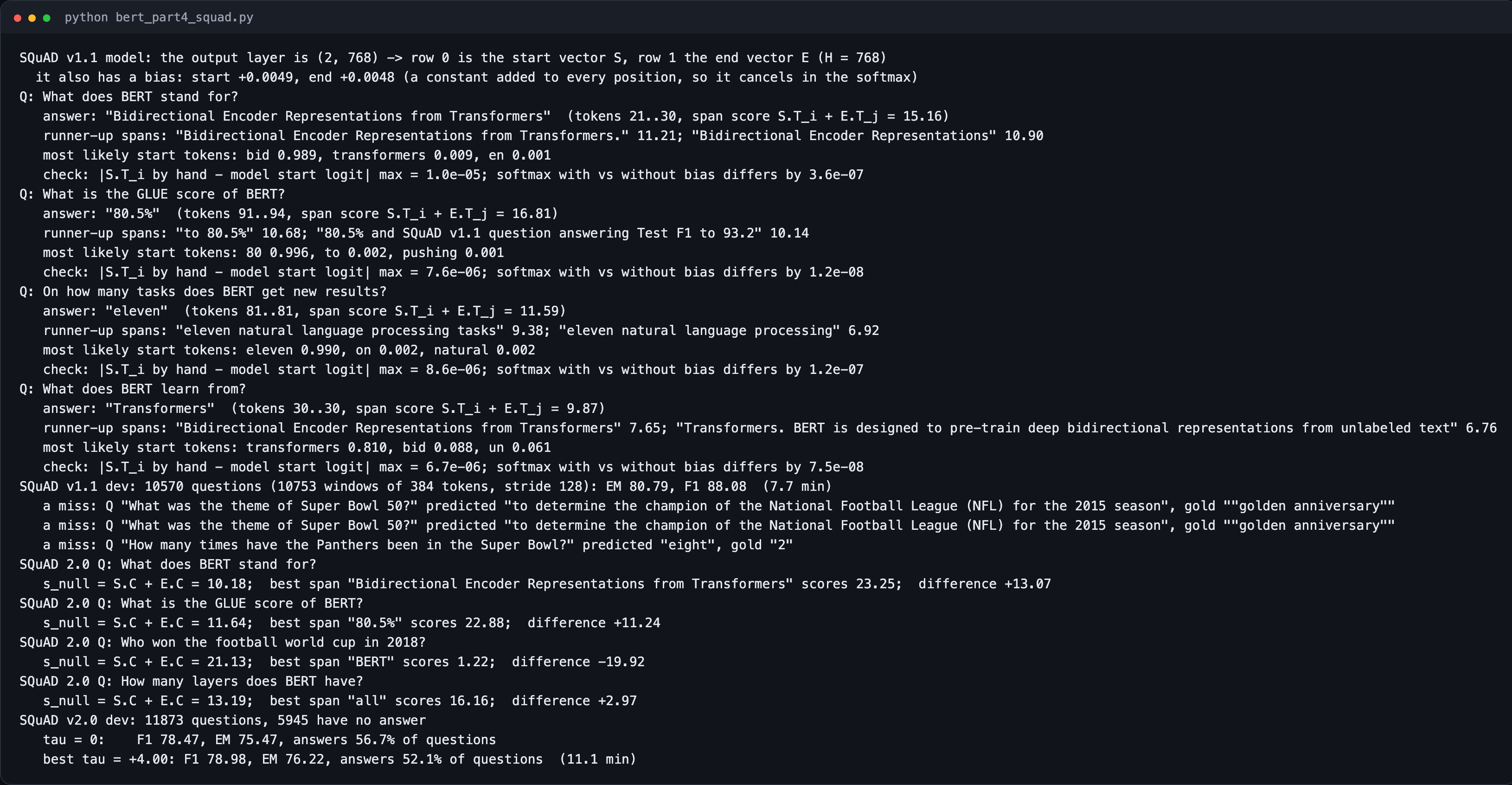
SQuAD v1.1 model: the output layer is (2, 768) -> row 0 is the start vector S, row 1 the end vector E (H = 768)
  it also has a bias: start +0.0049, end +0.0048 (a constant added to every position, so it cancels in the softmax)
Q: What does BERT stand for?
   answer: "Bidirectional Encoder Representations from Transformers"  (tokens 21..30, span score S.T_i + E.T_j = 15.16)
   runner-up spans: "Bidirectional Encoder Representations from Transformers." 11.21; "Bidirectional Encoder Representations" 10.90
   most likely start tokens: bid 0.989, transformers 0.009, en 0.001
   check: |S.T_i by hand - model start logit| max = 1.0e-05; softmax with vs without bias differs by 3.6e-07
Q: What is the GLUE score of BERT?
   answer: "80.5%"  (tokens 91..94, span score S.T_i + E.T_j = 16.81)
   runner-up spans: "to 80.5%" 10.68; "80.5% and SQuAD v1.1 question answering Test F1 to 93.2" 10.14
   most likely start tokens: 80 0.996, to 0.002, pushing 0.001
   check: |S.T_i by hand - model start logit| max = 7.6e-06; softmax with vs without bias differs by 1.2e-08
Q: On how many tasks does BERT get new results?
   answer: "eleven"  (tokens 81..81, span score S.T_i + E.T_j = 11.59)
   runner-up spans: "eleven natural language processing tasks" 9.38; "eleven natural language processing" 6.92
   most likely start tokens: eleven 0.990, on 0.002, natural 0.002
   check: |S.T_i by hand - model start logit| max = 8.6e-06; softmax with vs without bias differs by 1.2e-07
Q: What does BERT learn from?
   answer: "Transformers"  (tokens 30..30, span score S.T_i + E.T_j = 9.87)
   runner-up spans: "Bidirectional Encoder Representations from Transformers" 7.65; "Transformers. BERT is designed to pre-train deep bidirectional representations from unlabeled text" 6.76
   most likely start tokens: transformers 0.810, bid 0.088, un 0.061
   check: |S.T_i by hand - model start logit| max = 6.7e-06; softmax with vs without bias differs by 7.5e-08

Three things to notice:

• The formula is exactly the model. $S \cdot T_i$ computed by hand matches the model's start scores to about $10^{-5}$ (rounding noise of the GPU). The checkpoint also has a bias number added to every start score; adding the same number to every token does not change a softmax, and the output shows the probabilities differ by less than $10^{-6}$.
• "bid" is a word piece. The tokenizer cut "Bidirectional" into pieces (Part 2), and the answer starts at the first piece.
• It can be wrong. For "What does BERT learn from?", the model answered "Transformers". The right answer, "unlabeled text", is in the passage, but the phrase "Representations from Transformers" fooled it. Fine-tuned models match patterns; they do not reason like a reader.

Scoring on the full SQuAD v1.1 dev set#

One passage proves nothing about quality. So I ran the same checkpoint, with my own span search, on all questions of the SQuAD v1.1 dev set, using the official answer normalisation (lower case, no punctuation, no "a/an/the").

Written out, for one prediction and one gold answer, after normalising both (lowercase, remove punctuation and the words "a", "an", "the"):

When a question has several human answers, the score against the best-matching one counts. Worked examples:

pred "Bidirectional Encoder Representations" | gold "Bidirectional Encoder Representations from Transformers"
   shared words 3, precision 1.000, recall 0.600, F1 0.750, EM 0
pred "the Broncos defeated the Panthers" -> "broncos defeated panthers" | gold "Denver Broncos" -> "denver broncos"
   shared words 1, precision 0.333, recall 0.500, F1 0.400, EM 0

For the first: $F_1 = 2 \times 1 \times 0.6 / (1 + 0.6) = 0.75$.

Long passages do not fit in 384 tokens, so each one is cut into overlapping windows with a stride of 128 tokens (the settings of the released code), and the best span over all windows wins.

SQuAD v1.1 dev: 10570 questions (10753 windows of 384 tokens, stride 128): EM 80.79, F1 88.08  (9.3 min)
   a miss: Q "What was the theme of Super Bowl 50?" predicted "to determine the champion of the National Football League (NFL) for the 2015 season", gold ""golden anniversary""
   a miss: Q "What was the theme of Super Bowl 50?" predicted "to determine the champion of the National Football League (NFL) for the 2015 season", gold ""golden anniversary""
   a miss: Q "How many times have the Panthers been in the Super Bowl?" predicted "eight", gold "2"

On all 10,570 dev questions, this checkpoint with my decoding scores EM 80.79 and F1 88.08. Table 2 (next) lists 80.8 EM and 88.5 F1 for the authors' own BERT-base on the same dev set. So a BERT-base fine-tuned by someone else, decoded by my 60 lines of span search, lands within half a point of the paper. (The checkpoint's model page reports EM 80.91 and F1 88.23 with its own evaluation code; the small gap is down to decoding details such as how many candidate spans are tried.)

The misses are instructive. "What was the theme of Super Bowl 50?" appears twice because the dev set really contains two copies of that question (two separate entries with slightly different gold answers); both times the model picked a long span about the purpose of the game instead of "golden anniversary". And for "How many times have the Panthers been in the Super Bowl?" it answered "eight" where the answer is "2": a number from the right paragraph, attached to the wrong fact.

Table 2#

Two footnotes qualify Table 2:

The arithmetic: the ensemble's 93.2 test F1 minus the top leaderboard ensemble's 91.7 is the "+1.5". And the single model with TriviaQA (91.8 test F1) beats that top ensemble (91.7), which is the sentence "our single BERT model outperforms the top ensemble system in terms of F1 score".

SQuAD v2.0: when there is no answer#

The decision rule, written out:

where:

• $s_{\text{null}} = S \cdot C + E \cdot C$ is the score of the "span" that starts and ends at [CLS] (recall that $C$ is the final vector of [CLS]);
• $\hat{s}_{i,j}$ is the score of the best real span inside the passage, with $j \ge i$;
• $\tau$ (the Greek letter tau) is a threshold: a number you choose. A larger $\tau$ makes the model more careful (it answers less often).

Again I used a public checkpoint, deepset/bert-base-uncased-squad2 (BERT-base fine-tuned on SQuAD 2.0 by its authors, not by me), and computed both scores myself for two answerable and two unanswerable questions about the same abstract:

s_null = start[0] + end[0]                 # S.C + E.C: [CLS] is token 0
s_hat, i, j = best_span(start, end, passage_tokens)
answer = passage[i..j] if s_hat > s_null + tau else "no answer"

SQuAD 2.0 Q: What does BERT stand for?
   s_null = S.C + E.C = 10.18;  best span "Bidirectional Encoder Representations from Transformers" scores 23.25;  difference +13.07
SQuAD 2.0 Q: What is the GLUE score of BERT?
   s_null = S.C + E.C = 11.64;  best span "80.5%" scores 22.88;  difference +11.24
SQuAD 2.0 Q: Who won the football world cup in 2018?
   s_null = S.C + E.C = 21.13;  best span "BERT" scores 1.22;  difference -19.92
SQuAD 2.0 Q: How many layers does BERT have?
   s_null = S.C + E.C = 13.19;  best span "all" scores 16.16;  difference +2.97

The rule with real numbers, from a public BERT-base fine-tuned on SQuAD 2.0 (deepset/bert-base-uncased-squad2), on our BERT-abstract passage, with $\tau = 4.00$ chosen on the dev set (next section):

Q: What does BERT stand for?
   s_null = S.C + E.C = 5.08 + 5.10 = 10.18
   best span "Bidirectional Encoder Representations from Transformers": S.T_i + E.T_j = 11.69 + 11.56 = 23.25
   tau = +4.00: 23.25 > 14.18 ?  yes -> answer
Q: Who won the football world cup in 2018?
   s_null = S.C + E.C = 10.51 + 10.63 = 21.13
   best span "BERT": S.T_i + E.T_j = 0.33 + 0.89 = 1.22
   tau = +4.00: 1.22 > 25.13 ?  no -> no answer
Q: How many layers does BERT have?
   s_null = S.C + E.C = 6.61 + 6.58 = 13.19
   best span "all": S.T_i + E.T_j = 8.45 + 7.71 = 16.16
   tau = 0:     16.16 > 13.19 ?  yes -> answer
   tau = +4.00: 16.16 > 17.19 ?  no -> no answer

The last question shows what $\tau$ is for. The abstract does not say how many layers BERT has, and the best span ("all") is nonsense. With $\tau = 0$ the model would answer it; with $\tau = 4$ it correctly declines.

Read the differences:

• For the two answerable questions, the best span beats the no-answer score easily (+13.07 and +11.24).
• For the football question, nothing in the passage fits: the best span ("BERT") scores only 1.22, while [CLS] scores 21.13. The model says "no answer", which is right.
• The last question is the interesting one. "How many layers does BERT have?" sounds like it should be answerable, but the abstract never says. With $\tau = 0$ the model answers "all" (from "in all layers"), because that span beats $s_{\text{null}}$ by +2.97. That is a confident wrong answer, and exactly the kind of mistake the threshold $\tau$ exists to reduce: with $\tau$ above 2.97, the model would abstain.

Choosing τ on the dev set#

The paper picks $\tau$ "on the dev set to maximize F1". I did exactly that on the full SQuAD 2.0 dev set: for every question, store $\hat{s}_{i,j} - s_{\text{null}}$, then try thresholds from -6 to +6 in steps of 0.25.

SQuAD v2.0 dev: 11873 questions, 5945 have no answer
   tau = 0:    F1 78.47, EM 75.47, answers 56.7% of questions
   best tau = +4.00: F1 78.98, EM 76.22, answers 52.1% of questions  (8.2 min)

Of the 11,873 dev questions, 5,945 have no answer. With $\tau = 0$, the checkpoint gets F1 78.47. The best threshold on this dev set is $\tau = +4.00$, which gives F1 78.98 (EM 76.22) and makes the model answer 52.1% of the questions. The paper only reports BERT-large on SQuAD 2.0 (81.9 dev F1 in Table 3), so there is no BERT-base number to compare with directly; the checkpoint's model page reports 78.62 F1 with its own evaluation code.

One caution, which applies to the paper too: choosing $\tau$ on the dev set and then reporting the dev score flatters the dev score a little. That is why the paper's headline number is the test score, computed by the SQuAD organisers on hidden answers with the $\tau$ chosen on dev.

Table 3#

SWAG: choosing the best ending#

The scoring, written out for the four choices $k = 1, \dots, 4$:

where $C_k$ is the [CLS] vector when BERT reads "sentence + ending $k$", $w$ is the one new vector (768 numbers), and the softmax runs across the four choices. Unlike GLUE, the softmax is not over labels of one input, but over four separate inputs.

A toy example with $H = 4$: four [CLS] vectors and one learned vector $w = (2, -1, 0.5, 1)$:

Softmax over the four scores gives $(0.596,\ 0.015,\ 0.327,\ 0.063)$. If ending 1 is right, the loss is $-\log 0.596 = 0.518$.

The head in code, checked against BertForMultipleChoice (untrained, so the probabilities mean nothing yet; the point is the shapes and the arithmetic):

e = tok([ctx] * 4, endings, return_tensors="pt", padding=True)
e = {k: v.unsqueeze(0) for k, v in e.items()}                # (1 example, 4 choices, tokens)
C = model.bert(**{k: v.view(4, -1) for k, v in e.items()}).pooler_output   # (4, 768)
scores = C @ model.classifier.weight.T + model.classifier.bias           # (4, 1): one score each
probs = torch.softmax(scores.view(1, 4), -1)                 # softmax across the 4 choices

SWAG input: (1, 4, 16) = (batch, 4 choices, tokens); the vector w: (1, 768)
scores C.w by hand: [-0.3572, 0.141, -0.337, -0.0369];  library: [-0.3572, 0.141, -0.337, -0.0369]
softmax over the 4 choices (untrained w): [0.198, 0.326, 0.202, 0.273]

A careful reading note: SWAG was released in 2018 and built to be hard for the models of its day (its authors filtered out endings that their own models found easy, a method they call Adversarial Filtering). Within months, a fine-tuned BERT came close to human scores on it. This pattern (a benchmark is published, a bigger pre-trained model nearly solves it) repeated many times after BERT.

Next, in Part 5: the ablation studies. Is next sentence prediction really needed? How much of the gain is reading both ways? Do bigger models keep helping? And can BERT be used without fine-tuning at all, as a feature extractor?

Run it yourself

Three scripts produce every number in this part, in code/papers/bert/:

bashCopy

pip install torch transformers datasets
python bert_part4_heads.py            # the GLUE and SWAG heads checked by hand (CPU, seconds)
python bert_part4_finetune.py sst2    # fine-tune BERT-base on SST-2 (GPU recommended)
python bert_part4_finetune.py mrpc 2e-5   # MRPC with one learning rate; try 5e-5, 4e-5, 3e-5 too
python bert_part4_squad.py            # span search, SQuAD v1.1 and v2.0 dev sets (public checkpoints)

References#

The BERT paper

1. J. Devlin, M.-W. Chang, K. Lee, K. Toutanova. BERT: Pre-training of Deep Bidirectional Transformers for Language Understanding. NAACL 2019 (ACL Anthology).
2. Google Research. BERT code (run_classifier.py, run_squad.py, modeling.py).

Papers the BERT paper cites in this part

3. A. Wang, A. Singh, J. Michael, F. Hill, O. Levy, S. R. Bowman. GLUE: A Multi-Task Benchmark and Analysis Platform for Natural Language Understanding. BlackboxNLP workshop at EMNLP 2018.
4. A. Williams, N. Nangia, S. R. Bowman. A Broad-Coverage Challenge Corpus for Sentence Understanding through Inference (MultiNLI). NAACL 2018.
5. R. Socher et al. Recursive Deep Models for Semantic Compositionality Over a Sentiment Treebank (SST-2). EMNLP 2013.
6. A. Warstadt, A. Singh, S. R. Bowman. Neural Network Acceptability Judgments (CoLA). TACL 2019.
7. D. Cer, M. Diab, E. Agirre, I. Lopez-Gazpio, L. Specia. SemEval-2017 Task 1: Semantic Textual Similarity Multilingual and Crosslingual Focused Evaluation (STS-B). SemEval 2017.
8. W. B. Dolan, C. Brockett. Automatically Constructing a Corpus of Sentential Paraphrases (MRPC). IWP 2005.
9. L. Bentivogli, B. Magnini, I. Dagan, H. T. Dang, D. Giampiccolo. The Fifth PASCAL Recognizing Textual Entailment Challenge (RTE). TAC 2009.
10. H. J. Levesque, E. Davis, L. Morgenstern. The Winograd Schema Challenge (WNLI). KR 2012 (cited as an AAAI spring symposium paper, 2011).
11. P. Rajpurkar, J. Zhang, K. Lopyrev, P. Liang. SQuAD: 100,000+ Questions for Machine Comprehension of Text. EMNLP 2016.
12. P. Rajpurkar, R. Jia, P. Liang. Know What You Don't Know: Unanswerable Questions for SQuAD (SQuAD 2.0). ACL 2018.
13. M. Joshi, E. Choi, D. S. Weld, L. Zettlemoyer. TriviaQA: A Large Scale Distantly Supervised Challenge Dataset for Reading Comprehension. ACL 2017.
14. R. Zellers, Y. Bisk, R. Schwartz, Y. Choi. SWAG: A Large-Scale Adversarial Dataset for Grounded Commonsense Inference. EMNLP 2018.
15. A. P. Parikh, O. Täckström, D. Das, J. Uszkoreit. A Decomposable Attention Model for Natural Language Inference. EMNLP 2016.
16. M. Seo, A. Kembhavi, A. Farhadi, H. Hajishirzi. Bidirectional Attention Flow for Machine Comprehension (BiDAF). ICLR 2017.
17. A. W. Yu et al. QANet: Combining Local Convolution with Global Self-Attention for Reading Comprehension. ICLR 2018.
18. A. Radford, K. Narasimhan, T. Salimans, I. Sutskever. Improving Language Understanding by Generative Pre-Training (OpenAI GPT). OpenAI, 2018.

Other sources used in this part

19. Public checkpoints: csarron/bert-base-uncased-squad-v1, deepset/bert-base-uncased-squad2 and textattack/bert-base-uncased-SST-2.
20. Code for this part: bert_part4_heads.py, bert_part4_finetune.py, bert_part4_squad.py, bert_part4_math.py.