DeepSeek-R1, explained · Background · Covers Radford et al. 2018, Wei et al. 2022, Wang et al. 2022, Ouyang et al. 2022, Schulman et al. 2017, Lightman et al. 2023, Shao et al. 2024, DeepSeek-V3 2024
The Road to R1
How a language model learns, how it was taught to show its steps, and how reinforcement learning with human feedback works. The ideas the R1 paper assumes, with small runs you can check.
DeepSeek-R1: Incentivizing Reasoning Capability in LLMs via Reinforcement Learning. Daya Guo, Dejian Yang, Haowei Zhang, Junxiao Song, and others. arXiv 2025 (Nature 2025), 2025. arXiv:2501.12948
The R1 paper fits its method into two pages because it assumes that you know eight years of work before it. This page tells that story in class order, with the one equation that each idea stands on and a small run that you can check.
The story has one question. A language model can write fluent text. How do you make it think before it answers, and how do you train that skill when nobody can show it good thinking?
How a language model learns
Every model on this page starts the same way. It reads a huge amount of text and learns one skill: guess the next token. GPT-1 wrote this down in 2018, and the equation has not changed since.
We usually write the same idea as a loss that goes down, the cross-entropy. For a text of tokens:
Read it from the right. is the probability that the model, with weights , gives to the token that really came next. The log of a probability is negative, so the minus sign makes each term positive, and we take the mean. A perfect guess costs .
A tiny example by hand. Say the model gives the three right tokens the probabilities 0.5, 0.25 and 0.9. The costs are , and . The loss is their mean, 0.728. The unsure middle guess costs the most.
The loss in code
Our Method 1 writes the loss out: shift by one position, take a stable log-softmax by hand, and pick the probability of the right token. Method 2 is PyTorch's F.cross_entropy, and the model's own loss. We run both on Qwen2.5-0.5B, a small base model.
def next_token_loss(logits, ids):
    """Method 1: the next-token cross-entropy written out.
    logits: (T, V) scores at each position; ids: (T,) the tokens. Position t predicts token t + 1."""
    pred = logits[:-1]                                   # (T-1, V): the guesses for tokens 1..T-1
    target = ids[1:]                                     # (T-1,):   the tokens that really came next
    m = pred.max(dim=-1, keepdim=True).values            # subtract the max so exp() cannot overflow
    log_z = m.squeeze(-1) + torch.log(torch.exp(pred - m).sum(-1))   # (T-1,): log of the softmax denominator
    log_p = pred.gather(-1, target[:, None]).squeeze(-1) - log_z     # (T-1,): log p(right token)
return -log_p, -log_p.mean() # per-token losses and their mean per_tok, ours = next_token_loss(logits, ids[0])
lib = F.cross_entropy(logits[:-1], ids[0, 1:]) # Method 2== 1. Next-token loss of Qwen2.5-0.5B (base model) on one sentence
sentence: 'The capital of France is Paris, and the capital of Italy is Rome.'
tokens T = 15, vocabulary V = 151,936, logits shape (15, 151936)
next token p(next) -log p
' capital' 0.0001 9.317
' of' 0.5409 0.614
' France' 0.0416 3.179
' is' 0.7210 0.327
' Paris' 0.3156 1.153
',' 0.2210 1.509
' and' 0.1819 1.705
' the' 0.2121 1.551
' capital' 0.1571 1.851
' of' 0.9671 0.033
' Italy' 0.0438 3.128
' is' 0.9876 0.013
' Rome' 0.9232 0.080
'.' 0.6554 0.423
mean loss, ours (Method 1) : 1.7773
mean loss, F.cross_entropy (Method 2) : 1.7773
mean loss, model(ids, labels=ids).loss : 1.7773
max |ours - library| per token: 9.5e-07
perplexity exp(loss) = 5.91; a uniform guess would give loss ln(V) = 11.93The three numbers agree, and each token differs by less than one millionth. Look at the column of probabilities. After "The", the word "capital" is a surprise, so it costs 9.3. But " Rome" gets 0.92, because by then the model has seen the pattern "the capital of X is Y" once. A loss of 1.78 means that the model is about as unsure as a choice among 6 tokens, not 151,936.
Supervised fine-tuning: from base model to chat model
To get a model that answers, people write example answers and train on them. This is supervised fine-tuning (SFT). It was step 1 of the recipe that made the first instruction-following GPT models.
SFT uses the same loss as pre-training, with one change. The data is a prompt and a response, and the loss counts only the response tokens. The model should learn to answer, not to write questions. In code, the prompt tokens get the label , and both methods skip them:
def sft_loss(logits, labels):
    """Method 1 for SFT: the same loss, but only where labels != -100 (the response tokens)."""
    per_tok, _ = next_token_loss(logits, labels.clamp(min=0))
    keep = (labels[1:] != -100).float()                  # (T-1,): 1 on response tokens, 0 on prompt tokens
return (per_tok * keep).sum() / keep.sum()== 2. SFT loss: the same loss, only on the response tokens
prompt 13 tokens (label -100), response 18 tokens
SFT loss, ours (Method 1) : 0.5647
SFT loss, F.cross_entropy(ignore_index=-100) : 0.5647
SFT loss, model(ids, labels=labels).loss : 0.5647
loss on every token (prompt too), for comparison : 1.1737All three give 0.5647. The loss on every token is twice as high, because the question itself is hard to predict. SFT ignores that part.
SFT has a cost that matters for R1. It needs good answers to copy, and for hard maths, thousands of long, correct, step-by-step solutions are slow and costly to write. The examples also shape what the model learns: it is trained to imitate them, not to find methods they do not show. A student can still end up better than the examples, but SFT alone gives no direct push in that direction.
Chain of thought: let the model write its steps
In early 2022, a Google team found that you can get much better answers with no training at all. You only show the model a few examples that write out their steps.
A second idea came two months later. If one chain of thought can go wrong, write many and take a vote.
The vote is one line of maths. Given sampled answers :
is 1 when sample gave the answer , and 0 otherwise. The sum counts the votes for , and picks the answer with the most votes. With five samples 18, 18, 16, 18, 20, the counts are 3, 1 and 1, so the vote says 18.
Thinking and voting on a small model
We tried both ideas on Qwen2.5-0.5B-Instruct, a chat model of half a billion parameters, with the first 30 GSM8K test questions. Method 1 reads the answer with our own pattern and counts the votes by hand. Method 2 uses the math-verify library to check answers and collections.Counter to count votes.
def vote(answers):
    """Method 1: majority vote by hand. Count each answer; the first one to reach the top count wins ties."""
    counts, best = {}, None
    for a in answers:
        if a is None:
            continue
        counts[a] = counts.get(a, 0) + 1
        if best is None or counts[a] > counts[best]:
            best = a
    return best


def vote_lib(answers):
    """Method 2: the same vote with collections.Counter."""
    c = Counter(a for a in answers if a is not None)
return c.most_common(1)[0][0] if c else None== Chain of thought and majority vote: Qwen/Qwen2.5-0.5B-Instruct, first 30 GSM8K test questions, device mps
direct: greedy, reply starts with 'The answer is ', max 16 new tokens; CoT: greedy, max 512; samples: 16 per question, temperature 0.7, max 512
our regex math-verify mean new tokens
direct answer (greedy) 1/30 1/30 7.9
step by step (greedy) 12/30 11/30 314.0
one sample (mean of 16) 7.8/30 7.2/30 342.1
majority vote of 1 samples 7/30
majority vote of 2 samples 7/30
majority vote of 4 samples 10/30
majority vote of 8 samples 11/30
majority vote of 16 samples 14/30
at least one of 16 right 21/30
vote by hand vs Counter: 0 differences over 5 values of k x 30 questions
regex vs math-verify: same verdict on 524 of 540 replies
example, question 17: gold 230; greedy CoT said 115; 16 samples said ['2', '2', '320', '294', '230', '460', '230', '230', '450', '240', '170', '185', '230', '150', '230', '80']; vote 230
generation time 540 s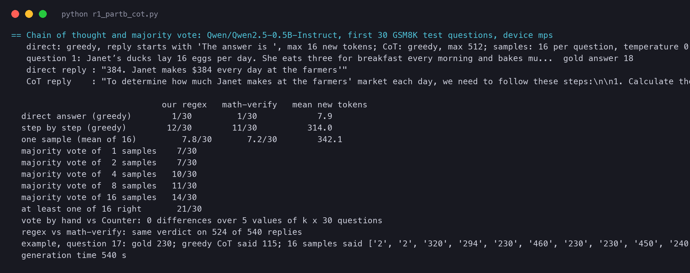
Read the table from the top. When the reply must start with "The answer is", the model is right on 1 question of 30. When it writes its steps first, it is right on 12.
One sampled chain (temperature 0.7) is right on 7.8 questions on average, fewer than the greedy chain. Sampling adds variety and also adds mistakes. But the vote turns that variety into accuracy: 10 with 4 samples, 11 with 8, and 14 with 16. Question 17 shows how. The greedy chain said 115; the 16 samples said many things, but 230, the right answer, came up 5 times and won.
Now look at the line "at least one of 16 right": 21 questions. The model can solve them, but not reliably. One way to read RL is as a method that moves the single answer toward the best sample.
Take these numbers as a demonstration, not a benchmark. 30 questions is a small sample, so one question moves the score by 3.3 points. The model is tiny, we cut chains at 512 tokens, and our answer reader and math-verify disagree on 16 of 540 replies. Our hand-written vote and Counter agree on all 150 votes.
Reinforcement learning, in the words of a language model
SFT needs an example of the right answer. Reinforcement learning (RL) needs only a score after the model acts. The model tries, a judge scores the try, and high-scoring tries become more likely. For maths, the judge can be a rule: is the final number right?
Here are the parts in the words of a language model. The policy is the model itself, with weights . A prompt is the situation. Each token that the model writes is one action. The full response is one episode, and the reward comes once, at the end. The goal is to make the average reward high:
We cannot take the gradient of a rule like "is the number right". But in 1992, Williams showed a way around it, the REINFORCE estimate. Sample a response, then push its log-probability up in proportion to its reward:
Read the left formula. is the direction that makes this response more likely. says how far to go, and in which direction. is a baseline, a number that does not depend on the response. The right formula says that the log-probability of a response is the sum over its tokens. So every token of the response gets the same push.
Why a baseline helps
Our tiny "model" picks one of four answers with probabilities 0.3875, 0.235, 0.1425 and 0.235. Only answer 2 is right, with reward 1. For a softmax policy, is "one-hot of minus ". So a sample of answer 2 gives the update : up for answer 2, down for the rest. A wrong sample has reward 0 and changes nothing.
Now add 5 to every reward. The true gradient does not change, because only differences matter. But a wrong answer now gets pushed up with weight 5, and only on average do the right answers win. A baseline near the mean reward takes the 5 away again. Here is the check, with 200,000 samples:
def grad_log_pi(theta, a):
    """Method 1: d log pi(a) / d theta for a softmax policy = one_hot(a) - pi.   (4,)"""
    g = -softmax(theta)
    g[a] += 1.0
return g g = (r - b)[:, None] * glp # (S, 4): one REINFORCE estimate per sample
mean = g.mean(0)
var = g.var(0).sum() # total variance over the 4 entries== 1. REINFORCE: a policy picks one of 4 answers; only answer 2 is right (reward 1, else 0)
pi = [0.3875, 0.235, 0.1425, 0.235] expected reward J = 0.1425
exact gradient dJ/dtheta = pi * (r - J) = [-0.0552, -0.0335, 0.1222, -0.0335]
grad log pi(a=2): ours [-0.3875, -0.235, 0.8575, -0.235] autograd [-0.3875, -0.235, 0.8575, -0.235]
exact gradient by autograd [-0.0552, -0.0335, 0.1222, -0.0335]
rewards +0, no baseline : mean of 200,000 estimates [-0.0554, -0.0336, 0.1227, -0.0336] variance 0.1221
rewards +0, baseline b = J : mean of 200,000 estimates [-0.0554, -0.0338, 0.1226, -0.0334] variance 0.0961
rewards +5, no baseline : mean of 200,000 estimates [-0.0554, -0.0272, 0.1254, -0.0428] variance 19.5260
rewards +5, baseline b = J : mean of 200,000 estimates [-0.0554, -0.0338, 0.1226, -0.0334] variance 0.0961Method 2, PyTorch's autograd, gives the same and the same exact gradient as our formulas. All four estimates have the right mean, up to sampling noise, because is zero on average. But the variance falls from 0.1221 to 0.0961 with 0/1 rewards, and from 19.5 to 0.0961 with shifted rewards.
Variance decides whether training works. We trained the same tiny policy for 300 steps, one sample per step, with 200 random seeds:
  rewards +0, no baseline     : step 50 mean 0.332, step 300 mean 0.960, worst seed 0.950, seeds below 0.5 at the end 0/200
  rewards +0, baseline        : step 50 mean 0.332, step 300 mean 0.959, worst seed 0.927, seeds below 0.5 at the end 0/200
  rewards +5, no baseline     : step 50 mean 0.270, step 300 mean 0.428, worst seed 0.001, seeds below 0.5 at the end 112/200
rewards +5, baseline : step 50 mean 0.333, step 300 mean 0.953, worst seed 0.872, seeds below 0.5 at the end 0/200With a baseline, every run learns. A baseline is not required: REINFORCE is correct without one, as the unshifted run shows. But it can cut the noise a great deal: from 19.5 to 0.0961 with shifted rewards. So most RL methods for language models use one, and the question is where it comes from. PPO learns it with a second network. GRPO takes it from a group of answers.
RLHF: learning from human rankings
For most prompts, no rule can say if an answer is good. Is this poem nice? Is this email polite? Step 2 of InstructGPT trains a model to give that score. People see several answers to one prompt and rank them, and a reward model learns to agree with them.
A tiny example. The reward model gives the winner 1.2 and the loser 0.4. The difference is 0.8, , and the loss is . If the scores were the other way round, the loss would be 1.171, so training pushes them apart. Method 1 is the formula; Method 2 is PyTorch's F.logsigmoid and F.binary_cross_entropy_with_logits:
== 2. Reward model (Bradley-Terry): loss = -log sigmoid(r(x, y_w) - r(x, y_l))
  r_w = 1.2, r_l = 0.4: P(w beats l) = 0.690, loss ours 0.3711  logsigmoid 0.3711  BCE-with-logits 0.3711
  r_w = 0.4, r_l = 1.2: P(w beats l) = 0.310, loss ours 1.1711  logsigmoid 1.1711  BCE-with-logits 1.1711
  r_w = 3.0, r_l = 0.0: P(w beats l) = 0.953, loss ours 0.0486  logsigmoid 0.0486  BCE-with-logits 0.0486
  ranking D > B > A > C -> 6 pairs: [('D', 'B'), ('D', 'A'), ('D', 'C'), ('B', 'A'), ('B', 'C'), ('A', 'C')]
  learned scores {'A': -1.35, 'B': 1.35, 'C': -4.33, 'D': 4.33}, final loss 0.029
  add 10 to every score: loss 0.029 (only differences count)
The last three lines learn four scores from one ranking, D > B > A > C, and they come out in that order. Adding 10 to every score leaves the loss the same. So a reward model has no natural zero, and InstructGPT shifts its scores before RL.
Step 3: raise the score, but stay close
Now the policy writes answers, the reward model scores them, and RL raises the score. But the reward model is only a guess of what people like. Far from familiar text, the policy can find odd answers that score high and that people dislike.
The reward that RL sees, from the paper's Equation 2 (we drop the term that mixes in pre-training data), is:
is the reward model's score. The log ratio is large when the policy makes this response much more likely than the SFT model did; this is the KL penalty. sets the length of the leash: InstructGPT uses (Appendix C.4). Spread over tokens, each token pays for its own probability:
== 3. RLHF reward with a per-token KL penalty: r_t = -beta * log(pi(t) / pi_ref(t)), plus r_RM at the end
  beta = 0.02 (InstructGPT, App. C.4), reward model score 1.5 on the last token
  token 1: pi 0.60  pi_ref 0.30  penalty ours -0.0139  torch -0.0139
  token 2: pi 0.90  pi_ref 0.90  penalty ours -0.0000  torch -0.0000
  token 3: pi 0.30  pi_ref 0.40  penalty ours +0.0058  torch +0.0058
  total reward = 1.5 + (-0.0139 + -0.0000 + +0.0058) = 1.4919
Token 1 doubled its probability compared with the reference, so it pays 0.0139. Token 2 did not move, so it pays nothing. Token 3 gets a small bonus, but on average the cost is never below zero: the mean log ratio is the KL divergence. The frozen SFT model that gives is called the reference model.
PPO: small, safe steps
The last piece is the update rule. Plain REINFORCE uses each batch of samples once, because a large step on old samples can wreck the policy. Proximal Policy Optimization (PPO, 2017) lets you reuse a batch for several steps, and it stops each step from going too far.
Our Method 1 is the formula with Python's min and max. Method 2 is torch.min and torch.clamp, and autograd tells us which terms still push:
def ppo_term(ratio, A, eps=0.2):
    """Method 1: one term of L_CLIP by hand."""
    clipped = min(max(ratio, 1 - eps), 1 + eps)
return min(ratio * A, clipped * A) lib = torch.min(rt * A, torch.clamp(rt, 1 - eps, 1 + eps) * A) # Method 2== 4. PPO clipped objective, epsilon = 0.2: min(ratio * A, clip(ratio, 0.8, 1.2) * A)
A = +1, ratio 0.5: unclipped +0.50 ours +0.50 torch +0.50 gradient +1
A = +1, ratio 0.9: unclipped +0.90 ours +0.90 torch +0.90 gradient +1
A = +1, ratio 1.0: unclipped +1.00 ours +1.00 torch +1.00 gradient +1
A = +1, ratio 1.1: unclipped +1.10 ours +1.10 torch +1.10 gradient +1
A = +1, ratio 1.5: unclipped +1.50 ours +1.20 torch +1.20 gradient +0
A = -1, ratio 0.5: unclipped -0.50 ours -0.80 torch -0.80 gradient +0
A = -1, ratio 0.9: unclipped -0.90 ours -0.90 torch -0.90 gradient -1
A = -1, ratio 1.0: unclipped -1.00 ours -1.00 torch -1.00 gradient -1
A = -1, ratio 1.1: unclipped -1.10 ours -1.10 torch -1.10 gradient -1
A = -1, ratio 1.5: unclipped -1.50 ours -1.50 torch -1.50 gradient -1Read the gradient column. A good token at ratio 1.5 has already moved too far, so its gradient is 0. A bad token at ratio 0.5 has already dropped enough, so its gradient is 0 too. But a bad token at ratio 1.5, one that the update made more likely by mistake, keeps its full gradient. The clip stops greed, not repair.
The cost: four models in memory
Now count the models that RLHF with PPO keeps in memory. The policy is trained, and the reference model is a frozen copy of SFT. The reward model is frozen too, and the critic is trained. The critic is not small: InstructGPT used a 6B reward model and a 6B critic started from it (Appendix C.4).
How much memory is "substantial"? A common rule says that a model trained with Adam in mixed precision needs about 16 bytes per parameter. A frozen one needs 2. For a 7-billion-parameter policy, this is our estimate, not a measurement:
== 5. Memory estimate for RLHF with PPO on a 7B policy (rule of thumb, not a measurement)
  policy    :   112 GB  (trained)
  critic    :   112 GB  (trained)
  reference :    14 GB  (frozen)
  reward    :    14 GB  (frozen)
total 252 GB; without the critic 140 GB (44% less), before activations and the KV cache of generationDrop the critic and the bill falls by 44% in this estimate. Hold that thought. It is exactly the model that GRPO removes, and Part 2 shows how.
Outcome rewards, process rewards, and reward hacking
For maths, there is a choice about what to score. You can score only the final answer, or you can score every step of the working.
Reward hacking is a policy that gets a high score without doing the task. A learned reward model is only an imperfect copy of the real goal, and RL is very good at finding the gaps.
Thinking longer at answer time
Chain of thought and voting share one idea: you can buy better answers with more computation at answer time. This is called test-time compute. Our small run showed the cost. A chain of thought used about 314 tokens per answer, against 8 for a direct answer, and a vote of 16 costs 16 chains.
In September 2024, OpenAI released o1, a model that writes a long hidden chain of thought before each answer. It was much stronger on competition maths and code. OpenAI's announcement showed accuracy rising with more thinking time, but it did not publish how it trained the model.
DeepSeek's two pieces
Two earlier DeepSeek papers supply the parts that R1 is built from: an RL algorithm and a base model.
The question R1 answers
Put the pieces side by side. A base model already holds the pieces of reasoning, and chain of thought shows that writing steps helps. RL can raise any score that you can compute. PPO makes the steps safe, but its critic doubles the trained models. Learned reward models invite hacking. And o1 showed that long thinking at answer time pays off, without saying how.
All the code of this page is in three scripts. r1_partb_loss.py has the losses, and r1_partb_cot.py has the thinking and voting run. r1_partb_rl.py has REINFORCE, the reward model, the KL penalty, PPO and the memory estimate.
The paper and the code
Paper (arXiv 2501.12948) · Official repository · Our code for this series