How 800k answers written by R1 teach six small open models to reason with plain fine-tuning, and why this beat RL on the same model. We write the loss by hand and test a distilled 1.5B model.
DeepSeek-R1: Incentivizing Reasoning Capability in LLMs via Reinforcement Learning. Daya Guo, Dejian Yang, Haowei Zhang, Junxiao Song, and others. arXiv 2025 (Nature 2025), 2025. arXiv:2501.12948
DeepSeek-R1 has 671 billion parameters, and few people can run it. Yet its reasoning can be copied into a 1.5-billion-parameter model that runs on a laptop. The small model needs no reinforcement learning: it only reads R1's written answers.
Background: what distillation is, and where it came from#
The word comes from chemistry. You boil a liquid, keep the vapour and cool it again, and you get the essence without the bulk. In machine learning, the "liquid" is a large model, and the "essence" is the behaviour we want a small model to copy.
Look at one position of a text. Let pT(v) be the teacher's probability that the next token is v, and pS(v) the student's. Word-level distillation uses the cross-entropy between the two lists:
Lword=−v∑pT(v)logpS(v)
Sequence-level distillation keeps only the token y^ that the teacher actually wrote at that position:
Lseq=−logpS(y^)
Read them from left to right. The sum runs over every token of the vocabulary. Each term is the teacher's probability for that token times the student's log-probability for it. The second loss has no sum: one token, one log-probability. Both are summed (or averaged) over all positions of the text.
A tiny example. Take a vocabulary of three tokens, A, B and C. The teacher gives (0.7, 0.2, 0.1) and the student gives (0.5, 0.3, 0.2). The word-level loss is
Suppose the teacher sampled A. The sequence-level loss is −ln0.5=0.693. If it had sampled C, the loss would be −ln0.2=1.609. Now sample many times from the teacher: A comes 70% of the time, B 20% and C 10%. The average sequence-level loss is then exactly 0.887, the word-level loss. Sampled text is a noisy but honest copy of the teacher's distribution.
R1's data is not plain samples either. For each prompt the authors sample several answers and keep only the correct ones (Part 5 runs this rejection sampling). Version 1 does not give the sampling temperature for this step; the 0.6 of §3 is for evaluation. So the student copies the teacher's good answers, not its full distribution. That is a choice, and it fits the goal: we want the student to reason well, not to copy R1's mistakes.
One real position of our duck trace, with R1-Distill-Qwen-1.5B as the teacher, seen both ways. On the left, the teacher's top five next tokens and their probabilities, which a word-level student would match. On the right, the one token that the sampled text keeps, which is all that an R1 student sees.
Why did DeepSeek choose the text and not the probabilities? Three reasons follow from the setup, although the paper does not list them. None of the six students uses R1's tokenizer, so R1's probabilities over its own tokens do not line up with a student's tokens. Storing a full probability list for every token of 800k long answers would be huge, while text is small. And the 800k samples already existed: they were made for R1's own training.
Distillation: fine-tune small models on R1's answers#
You are here. Part 5 turns DeepSeek-V3-Base into DeepSeek-R1, and its stage 3 builds 800k samples. Section 2.4 fine-tunes six open models on those samples, with no RL stage.
Every step of this SFT uses one loss. The intuition is a teacher who reads a student's essay aloud and asks, at each word, "how surprised were you by this word?". The student is graded only on the answer part, never on the question, because the question is given.
LSFT=−N1t∈response∑logpθ(yt∣y<t)
Read it from left to right. N is the number of response tokens. The sum runs only over positions in the response, the teacher's answer. yt is the token that the teacher wrote at position t, and y<t is everything before it, the prompt included. pθ is the student's probability, with its weights θ. The minus sign turns "high probability" into "low loss".
This is exactly the sequence-level loss of the last section, averaged over a whole answer. A tiny example: a response of three tokens that the student gives probabilities 0.5, 0.25 and 0.8. The loss is −(ln0.5+ln0.25+ln0.8)/3=(0.693+1.386+0.223)/3=0.767. The prompt tokens add nothing, however unlikely they are.
How does a program know which tokens are the response? Libraries mark every prompt token with the label −100, a number that no real token has, and skip those positions in the sum. The student must also predict token t+1 from position t, so the labels are shifted by one. These two details are where SFT code usually goes wrong, so we write them ourselves.
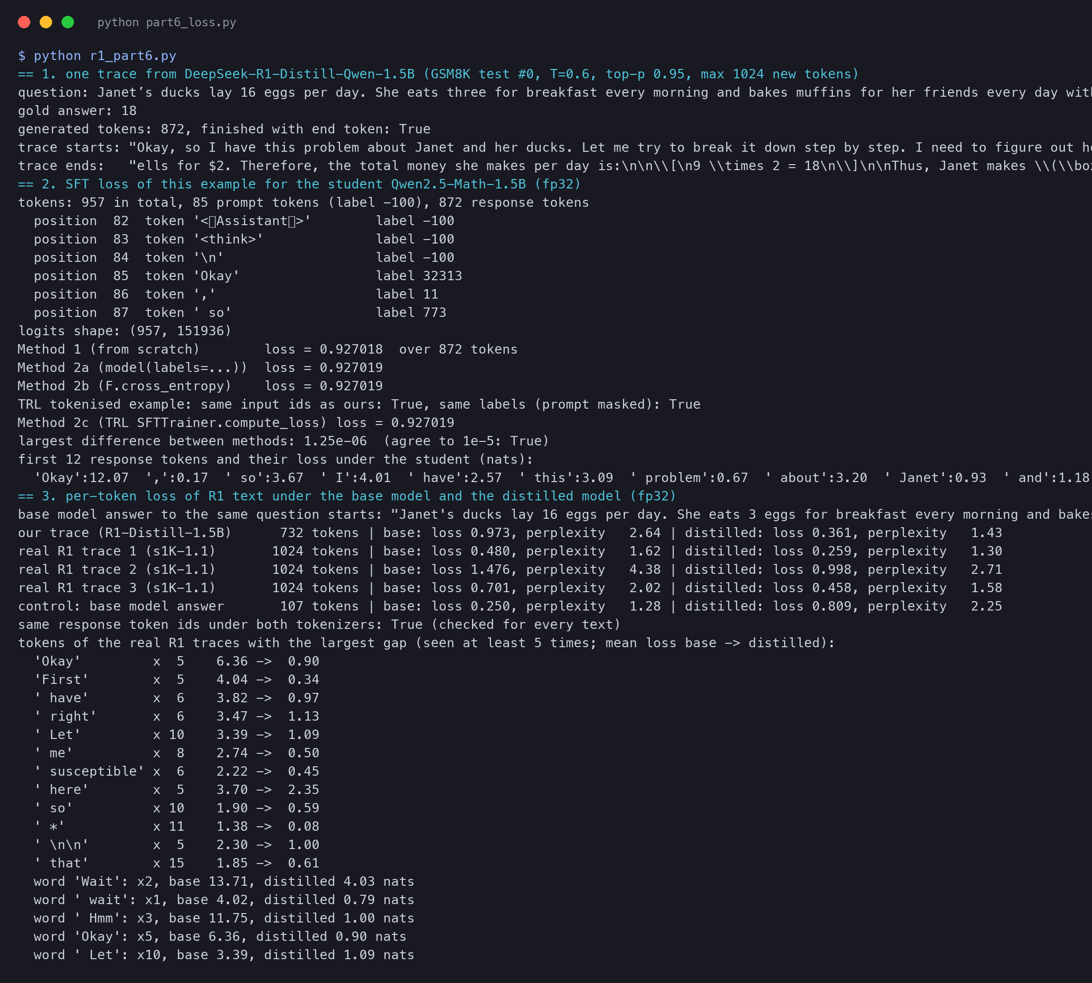
We use a real R1-style example. The distilled 1.5B model solved the first problem of the GSM8K test set, about a farmer's ducks and eggs:
plain text
question: Janet’s ducks lay 16 eggs per day. She eats three for breakfast every morning and bakes muffins for her friends every day with four. She sells the remainder at the farmers' market daily for $2 per fresh duck egg. How much in dollars does she make every day at the farmers' market?gold answer: 18generated tokens: 872, finished with end token: Truetrace starts: "Okay, so I have this problem about Janet and her ducks. Let me try to break it down step by step. I need to figure out how much money Janet makes every day at the farmers' market. Hmm, let's see.\n\nFirst, the problem says"trace ends: "ells for $2. Therefore, the total money she makes per day is:\n\n\\[\n9 \\times 2 = 18\n\\]\n\nThus, Janet makes \\(\\boxed{18}\\) dollars every day at the farmers' market."
Then we tokenise it the way SFT does. The prompt comes from the chat template and ends with the thinking tag; the response is the teacher's text plus the end token.
python
def build_example(tok, question, response):
    """Tokenise one distillation example the way SFT sees it.
    prompt: the chat template up to where the assistant starts (it ends with '<think>\\n' for the R1 template).
    response: the teacher's text plus the end-of-sequence token. Only the response is trained on."""
    msgs = [{'role': 'user', 'content': question + SUFFIX}]
    prompt_ids = tok.apply_chat_template(msgs, add_generation_prompt=True, tokenize=True)   # list of P ids
    if not isinstance(prompt_ids, list):
        prompt_ids = prompt_ids['input_ids']
    response_ids = tok(response + tok.eos_token, add_special_tokens=False)['input_ids']  # list of N ids
    input_ids = prompt_ids + response_ids                                                 # P + N ids
    labels = [-100] * len(prompt_ids) + response_ids                                      # -100 = "no loss here"
    return input_ids, labels, len(prompt_ids)
The tokens of our real example around the boundary between prompt and response. Prompt tokens carry the label minus 100; response tokens carry their own token id.
plain text
tokens: 957 in total, 85 prompt tokens (label -100), 872 response tokens
  position  82  token '<|Assistant|>'        label -100
  position  83  token '<think>'              label -100
  position  84  token '\n'                   label -100
  position  85  token 'Okay'                 label 32313
  position  86  token ','                    label 11
  position  87  token ' so'                  label 773
Now the loss itself, with the log-softmax written by hand. A model returns one row of scores (logits) for each position. The softmax turns a row into probabilities, and we need their log.
python
def sft_loss_from_scratch(logits, labels):
    """Method 1. logits: (T, V) floats, one row per position. labels: (T,) ids, -100 where there is no loss.
    The model at position t predicts the token at t + 1, so we shift by one."""
    logits = logits[:-1]                                      # (T-1, V): predictions made at positions 0 .. T-2
    target = labels[1:]                                       # (T-1,):   the tokens at positions 1 .. T-1
    keep = target != -100                                     # (T-1,):   True only on response tokens
    m = logits.max(dim=-1, keepdim=True).values               # (T-1, 1): row maximum, for a stable log-sum-exp
    logsumexp = m + torch.log(torch.exp(logits - m).sum(dim=-1, keepdim=True))   # (T-1, 1)
    logprobs = logits - logsumexp                             # (T-1, V): log-softmax by hand
    picked = logprobs[keep].gather(1, target[keep].unsqueeze(1)).squeeze(1)      # (N,): log p(correct token)
    nll = -picked                                             # (N,): loss of each response token
    return nll.mean(), nll                                    # mean over response tokens only
The student here is Qwen2.5-Math-1.5B, the base model that became R1-Distill-Qwen-1.5B. We give it the same example three more ways. transformers computes the loss itself when it gets labels. PyTorch's cross_entropy skips the −100 labels with ignore_index. And TRL's SFTTrainer, the trainer most people use for this job, tokenises the prompt and completion, builds its own labels and computes its own loss.
python
loss1, nll1 = sft_loss_from_scratch(logits, lab[0]) # Method 1, our function# Method 2a: transformers computes the loss itself when we pass labelsloss2 = bmodel(ids, labels=lab).loss.float()# Method 2b: PyTorch's cross_entropy with ignore_index=-100loss2b = F.cross_entropy(logits[:-1], lab[0, 1:], ignore_index=-100)# Method 2c: TRL's SFTTrainer builds the example (tokenise, mask the prompt) and computes the lossds = Dataset.from_list([{'prompt': prompt_text, 'completion': trace + dtok.eos_token}])cfg = SFTConfig(output_dir=os.path.join(RESULTS, '.part6_trl_tmp'), report_to=[], completion_only_loss=True, max_length=None, per_device_eval_batch_size=1)trainer = SFTTrainer(model=bmodel, args=cfg, train_dataset=ds, processing_class=dtok)ex = trainer.train_dataset[0]same_ids = list(ex['input_ids']) == input_idssame_labels = list(ex['labels']) == labelsbatch = trainer.data_collator([ex])loss3 = trainer.compute_loss(bmodel, {k: v.to(DEV) for k, v in batch.items()}).float()
plain text
logits shape: (957, 151936)Method 1 (from scratch) loss = 0.927018 over 872 tokensMethod 2a (model(labels=...)) loss = 0.927019Method 2b (F.cross_entropy) loss = 0.927019Method 2c (TRL SFTTrainer.compute_loss) loss = 0.927019TRL tokenised example: same input ids as ours: True, same labels (prompt masked): Truelargest difference between methods: 1.25e-06 (agree to 1e-5: True)first 12 response tokens and their loss under the student (nats): 'Okay':12.07 ',':0.17 ' so':3.67 ' I':4.01 ' have':2.57 ' this':3.09 ' problem':0.67 ' about':3.20 ' Janet':0.93 ' and':1.18 ' her':0.08 ' ducks':0.14
All four numbers are 0.927 nats per token. Our function and the libraries differ by 1.25×10⁻⁶, which is rounding in 32-bit floats, well inside 10−5. TRL also built exactly our token ids and exactly our labels, with the 85 prompt tokens masked. So the whole of SFT distillation fits in the two short functions above: build the labels, then average the log-probabilities of the response.
The per-token losses are worth a look. The base model gives the first word, "Okay", a loss of 12.07 nats: it almost never starts an answer like that. A few tokens later, " her" and " ducks" cost under 0.15 nats, because the question already said them. Distillation must teach the student the first kind of token, the voice and habits of R1. The second kind it already knows.
Table 5 drawn as bars: AIME 2024 pass@1 and MATH-500 pass@1 for the four comparison models (top) and the six distilled students (bottom).
R1-Distill-Qwen-1.5B. AIME 28.9, MATH-500 83.9, GPQA 33.8, LiveCodeBench 16.9, Codeforces 954. On the two maths tests it beats GPT-4o (9.3 and 74.6) and Sonnet 3.5 (16.0 and 78.3). On GPQA and LiveCodeBench it is far below both. GPQA Diamond has four choices per question, so 33.8% is not far above a guess.
On the Codeforces rating, the 1.5B student is above both chat models: 954 against 759 and 717. But that column measures competition problems, which are close to maths puzzles.
R1-Distill-Qwen-7B. AIME 55.5, MATH-500 92.8. On maths it is already near o1-mini (63.6 and 90.0) and above QwQ-32B-Preview on AIME (50.0). It beats GPT-4o on every column but one: GPQA, 49.1 against 49.9. The paper's words "across the board" round that away.
R1-Distill-Qwen-14B. AIME 69.7, cons@64 80.0, MATH-500 93.9, GPQA 59.1, LiveCodeBench 53.1, Codeforces 1481. Every one of these numbers is above QwQ-32B-Preview's, a model more than twice its size that was built to reason.
R1-Distill-Qwen-32B. AIME 72.6, MATH-500 94.3, GPQA 62.1, LiveCodeBench 57.2. It beats o1-mini on five of six columns. The exception is the Codeforces rating, 1691 against 1820.
R1-Distill-Llama-8B. AIME 50.4, MATH-500 89.1. It is a little weaker on maths than the Qwen 7B student, which started from a maths model. On code it is a little stronger: LiveCodeBench 39.6 against 37.6.
R1-Distill-Llama-70B. AIME 70.0, cons@64 86.7, MATH-500 94.5, GPQA 65.2, LiveCodeBench 57.5. It has the best value in four columns. Yet it is more than twice the size of the Qwen 32B student, and only level with it. AIME is 70.0 against 72.6, and MATH-500 is 94.5 against 94.3.
Two patterns run through the rows. First, size helps, but less and less: AIME goes 28.9, 55.5, 69.7, 72.6 from 1.5B to 32B. Second, the start matters. The maths models are strong on maths for their size. The Llama students are not better per parameter than the Qwen students.
GPT-4o, Sonnet 3.5 and the distilled 1.5B model on four benchmarks of Table 5. The 1.5B model is first on both maths tests and last on science and code.
Why the split? A small model has little room for facts. GPQA asks for deep knowledge of biology, physics and chemistry, and reasoning cannot make up for facts the model does not know. Maths problems need fewer facts and more steps, and steps are what R1's text teaches.
Section 1 says that the student copies R1's "reasoning patterns". We can measure that idea directly. Take text that R1 wrote, and ask two models how surprised they are by each token. One is the base model Qwen2.5-Math-1.5B, before distillation. The other is R1-Distill-Qwen-1.5B, after it. The loss is the same LSFT as above, so a lower number means "this is the kind of text I write".
We use five texts. One is the trace from above. Three are real traces of the full DeepSeek-R1, from the public s1K-1.1 dataset. We took the three shortest correct ones among its first 300 rows, cut at 1,024 tokens. The last one is a control: an answer that the base model wrote itself to the duck problem.
plain text
our trace (R1-Distill-1.5B) 732 tokens | base: loss 0.973, perplexity 2.64 | distilled: loss 0.361, perplexity 1.43real R1 trace 1 (s1K-1.1) 1024 tokens | base: loss 0.480, perplexity 1.62 | distilled: loss 0.259, perplexity 1.30real R1 trace 2 (s1K-1.1) 1024 tokens | base: loss 1.476, perplexity 4.38 | distilled: loss 0.998, perplexity 2.71real R1 trace 3 (s1K-1.1) 1024 tokens | base: loss 0.701, perplexity 2.02 | distilled: loss 0.458, perplexity 1.58control: base model answer 107 tokens | base: loss 0.250, perplexity 1.28 | distilled: loss 0.809, perplexity 2.25same response token ids under both tokenizers: True (checked for every text)
The mean loss per token of five texts under the base model and the distilled model. Lower means the model finds the text more likely.
The pattern is clear. On every R1-style text, the distilled model has the lower loss. On our trace it falls from 0.973 to 0.361 nats per token, so the perplexity falls from 2.64 to 1.43. On the three real R1 traces it falls from 0.480 to 0.259, from 1.476 to 0.998, and from 0.701 to 0.458.
The control row turns the other way. On the base model's own answer, the base model has a loss of 0.250 and the distilled model 0.809. So the distilled model is not simply "better at text". It has moved toward one style of text, R1's, and away from the plain answers the base model used to write.
Two notes keep the test honest. Our trace was written by the distilled model itself, so this model must find it likely. That is why the three real R1 traces matter. Also, we used only the thinking part of our trace, 732 tokens. The end-of-thinking tag is one token for the R1 tokenizer and several for the base one. Every text gave identical token ids under both tokenizers, which the script checks.
The loss of every token of a real R1 trace, smoothed, under the base model and the distilled model.
Which tokens moved most? The script averages the loss of each token over the three real R1 traces. It keeps tokens seen at least five times and sorts them by the drop:
plain text
tokens of the real R1 traces with the largest gap (seen at least 5 times; mean loss base -> distilled):
  'Okay'         x  5    6.36 ->  0.90
  'First'        x  5    4.04 ->  0.34
  ' have'        x  6    3.82 ->  0.97
  ' right'       x  6    3.47 ->  1.13
  ' Let'         x 10    3.39 ->  1.09
  ' me'          x  8    2.74 ->  0.50
  ' susceptible' x  6    2.22 ->  0.45
  ' here'        x  5    3.70 ->  2.35
  ' so'          x 10    1.90 ->  0.59
  ' *'           x 11    1.38 ->  0.08
  ' \n\n'        x  5    2.30 ->  1.00
  ' that'        x 15    1.85 ->  0.61
  word 'Wait': x2, base 13.71, distilled 4.03 nats
  word ' wait': x1, base 4.02, distilled 0.79 nats
  word ' Hmm': x3, base 11.75, distilled 1.00 nats
  word 'Okay': x5, base 6.36, distilled 0.90 nats
  word ' Let': x10, base 3.39, distilled 1.09 nats
The top of the list is not maths. It is the voice of a thinker talking to itself: "Okay", "First", " Let", " me", " right". The words that mark R1's self-checks move the most of all. "Wait" costs the base model 13.71 nats, which is a probability of about one in a million, and the distilled model 4.03. " Hmm" goes from 11.75 to 1.00. These are the "reasoning patterns" of §1, visible as numbers: the student learned when to stop, doubt and look again.
The paper scores six students on five benchmarks with up to 32,768 tokens per answer. We can do a small part of that: the same base model and its released student on the same maths problems. We drew 16 problems of levels 1 to 3 from MATH-500, with a fixed seed. Each model wrote 4 answers per problem, with temperature 0.6 and top-p 0.95 as in §3. Each answer may use at most 2,048 new tokens, 16 times less than the paper allows.
We grade with one policy, the same as in Part 4. An answer that hits the 2,048-token limit has no final answer, so it counts as wrong. For the distilled model, we grade only the text after </think>: the summary it writes once it has finished thinking. An answer that never closes </think> counts as wrong. The base model writes no thinking block, so we grade its whole finished text. math-verify then compares the last boxed answer with the reference.
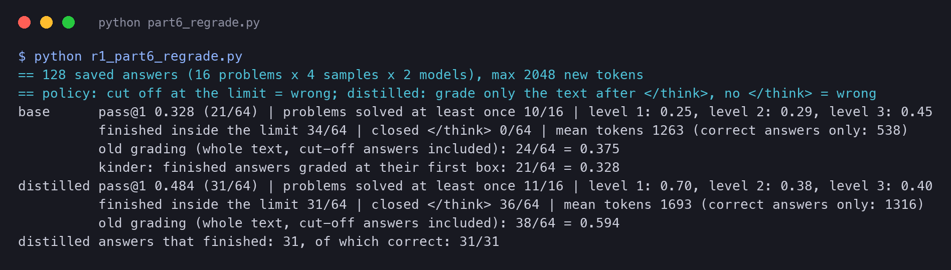
The generation script saved every answer, and r1_part6_regrade.py grades the saved answers with this policy. No model runs again:
plain text
$ python r1_part6_regrade.py== 128 saved answers (16 problems x 4 samples x 2 models), max 2048 new tokens== policy: cut off at the limit = wrong; distilled: grade only the text after </think>, no </think> = wrongbase pass@1 0.328 (21/64) | problems solved at least once 10/16 | level 1: 0.25, level 2: 0.29, level 3: 0.45 finished inside the limit 34/64 | closed </think> 0/64 | mean tokens 1263 (correct answers only: 538) old grading (whole text, cut-off answers included): 24/64 = 0.375 kinder: finished answers graded at their first box: 21/64 = 0.328distilled pass@1 0.484 (31/64) | problems solved at least once 11/16 | level 1: 0.70, level 2: 0.38, level 3: 0.40 finished inside the limit 31/64 | closed </think> 36/64 | mean tokens 1693 (correct answers only: 1316) old grading (whole text, cut-off answers included): 38/64 = 0.594distilled answers that finished: 31, of which correct: 31/31
Our run on 16 MATH-500 problems: accuracy under one grading policy (a cut-off answer is wrong, the distilled model is graded after its thinking), mean answer length, and answers that hit the 2,048-token limit, for the base model and the distilled model.
The distilled model is right on 31 of 64 answers, a pass@1 of 0.484. The base model is right on 21 of 64, or 0.328. The distilled model solves 11 of the 16 problems at least once; the base model solves 10. That is the direction of Table 5, on a much smaller test.
Look at the "old grading" lines. Our first grading read the whole text of every answer, cut off or not, and gave 38 and 24. That was too kind. A cut-off answer can hold a boxed number from the middle of its thinking, a step the model had not yet checked. The old grader counted it. The policy above does not.
The lengths tell the other half. The distilled model's correct answers average 1,316 tokens; the base model's correct answers average 538. The student has learned to think for a long time, as R1 does. With a cap of 2,048 tokens, 33 of its 64 answers were cut off before they ended.
Every one of the 31 answers that did finish was right. So the cap, not the model, decides most of this score. With the paper's 32,768 tokens, this model would likely score higher than 0.484.
The base model also hit the limit, 30 times, but for a different reason. We read its long answers. It often gives an answer and then keeps going. It writes a new problem of its own and solves that, or it repeats one phrase until the cap. A base model was never taught where an answer ends. Under our policy these answers are wrong, because they never end.
The "kinder" line grades each finished base answer at its first box instead of its last; it changes nothing (21 either way).
Sixteen problems with four samples each is a small test, so read these numbers as a direction, not as a benchmark score.
Table 6 as bars. On the same Qwen2.5-32B base, over 10K steps of RL give about the level of QwQ-32B-Preview; SFT on R1's 800k samples gives much more on every column.
Can we watch the recipe work at toy size? We tried §2.3.3 and §2.4 in miniature. The teacher was R1-Distill-Qwen-1.5B, standing in for R1. The student was Qwen2.5-0.5B-Instruct.
The teacher wrote one answer for each of 128 GSM8K training problems, with at most 1,024 new tokens. We kept only the answers that ended and were right. Then the student got SFT on the kept answers with our Method 1 loss. We used 3 epochs, batch 1, AdamW, and a learning rate of 10−5 with cosine decay to one tenth.
plain text
== 1. teacher deepseek-ai/DeepSeek-R1-Distill-Qwen-1.5B writes one trace per problem (128 GSM8K train problems, max 1024 tokens)== 0. teacher distribution at response position 444 (after " $18 every day at the farmers' market.\n\n"): 'Wait' 0.900, 'Let' 0.074, 'Hmm' 0.011, 'But' 0.005, 'Hold' 0.005; the trace has 'Wait' (p = 0.900)traces written 128, finished and correct (kept) 35, mean length of kept 835 tokens, 391 s== 3a. student Qwen/Qwen2.5-0.5B-Instruct before distillation (30 held-out GSM8K test problems x 2 samples)before accuracy 0.450 (27/60) | mean tokens 328 | with </think> 0/60 | with "Wait" 0/60 | hit the limit 0/60== 2. SFT on the kept traces: 3 epochs, batch 1, AdamW, lr 1e-05 cosine to 1.0000000000000002e-06 step 1/105 loss 0.8382 (mean of last 1) 3 s step 25/105 loss 0.7023 (mean of last 25) 52 s step 50/105 loss 0.4550 (mean of last 25) 162 s step 75/105 loss 0.3267 (mean of last 25) 476 s step 100/105 loss 0.1719 (mean of last 25) 712 s
The run did not finish. Our session was restarted at step 100 of 105, before the last evaluation, and the shared machine was then busy with a long training job. So we have no "after" numbers, and we do not guess them. What the log does show is still worth reading.
First, rejection sampling is expensive. Of 128 answers, only 35 both ended within 1,024 tokens and were right. Most of the rest were cut off while still thinking. The kept answers average 835 tokens, against 328 tokens for the student's own answers before training.
Second, the student starts far from the teacher's style. Before training it is right on 27 of 60 answers, and none of its 60 answers contains "Wait" or a thinking tag. Its training loss on the teacher's text then falls from 0.84 at the first step to 0.17 over steps 76 to 100. That fall is the same effect as in our comparison of the two 1.5B models: the student learns to find the teacher's text likely.
Third, the probe at the top of the log is the left half of the figure of the two losses. At one position of our duck trace, after the final answer, the teacher gives "Wait" a probability of 0.900, "Let" 0.074 and "Hmm" 0.011. The model checks its work even after it has the answer.