DeepSeek-R1, explained · Part 2 of 8 · Covers §2.1, §2.2, §2.2.1, Equations 1 to 3
GRPO: Learning from a Group of Answers
The learning rule behind DeepSeek-R1, term by term: sample a group of answers, score them, and push the model toward the better ones without a critic. We write GRPO from scratch, match it with TRL, and run one real step on a small model.
DeepSeek-R1: Incentivizing Reasoning Capability in LLMs via Reinforcement Learning. Daya Guo, Dejian Yang, Haowei Zhang, Junxiao Song, and others. arXiv 2025 (Nature 2025), 2025. arXiv:2501.12948
DeepSeek-R1-Zero learned to reason from one short rule: try a question many times, then make the better tries more likely. This page reads the three equations that turn that rule into training, slowly, with numbers you can check by hand and code that runs.
Three things the paper does
Learning without worked examples
To learn from scores, the model needs a rule that turns a score into a change of its weights. Reinforcement learning has a name for the model in this role.
Group Relative Policy Optimization
Background: the problem every policy-gradient method solves
Start with the simplest rule. The model writes an answer. If the reward is high, make every token of that answer a little more likely. If it is low, make them a little less likely. This is the policy gradient, and its basic form is "reward times the gradient of the log-probability of the answer".
A small example shows the weakness. Say rewards are 1 for a right answer and 0 for a wrong one. Then wrong answers get a push of 0: the model learns nothing from its mistakes. Now say a different task gives rewards between 8 and 10. Every answer gets a large positive push, even the worst one. The model learns slowly, because the useful signal (9.8 is better than 8.1) hides in a large shared number.
The fix is to subtract a baseline: a guess of the usual reward for this question. Then only "better than usual" gets a positive push and "worse than usual" gets a negative one. The difference has its own name.
The hard part is the baseline. A question that the model nearly always solves should have a high baseline, and a hard question a low one. Something must estimate it for each question. PPO trains a network for that.
The Road to R1 tells how PPO came to language models through human feedback. Here we need only its structure.
PPO and its critic
The later long version of the R1 paper adds a reason that matters for long reasoning.
How big is the saving? Our script counts the memory for the weights and the optimizer state only. A trained model with mixed-precision Adam keeps about 16 bytes per parameter (bf16 weights and gradients, fp32 master weights and two fp32 Adam moments). A frozen model that only runs forward needs 2 bytes per parameter. We assume the critic and the reward model have the same size as the policy.
== 7B policy: 7B parameters per model
PPO                  policy 112 + reference 14 + reward model 14 + value model 112 = 252 GB
GRPO, reward model   policy 112 + reference 14 + reward model 14 = 140 GB
GRPO, rule rewards   policy 112 + reference 14 = 126 GB
GRPO with rule rewards needs 50% of the memory of PPO; it saves 126 GB
80 GB GPUs just to hold these (rounded up): PPO 4, GRPO with rule rewards 2
the value model alone: 112 GB, 2 GPUs of 80 GB (rounded up)

== DeepSeek-V3 size: 671B parameters per model
PPO                  policy 10,736 + reference 1,342 + reward model 1,342 + value model 10,736 = 24,156 GB
GRPO, reward model   policy 10,736 + reference 1,342 + reward model 1,342 = 13,420 GB
GRPO, rule rewards   policy 10,736 + reference 1,342 = 12,078 GB
GRPO with rule rewards needs 50% of the memory of PPO; it saves 12,078 GB
80 GB GPUs just to hold these (rounded up): PPO 302, GRPO with rule rewards 151
the value model alone: 10,736 GB, 135 GPUs of 80 GB (rounded up)
For a model the size of DeepSeek-V3 (671 billion parameters, see the V3 architecture), the critic alone would take 10,736 GB in this count. That is 135 GPUs of 80 GB only to hold one network. R1-Zero also has no reward model: its rewards are rules in a program (Part 3). So GRPO in R1-Zero trains one large network and keeps one frozen copy. These numbers are a rough count. Real training adds activations and the memory for sampling, and DeepSeek uses FP8 and other savings.
Where GRPO came from
GRPO was not new in R1. DeepSeek introduced it a year earlier, in the DeepSeekMath paper, to train a 7B maths model.
Here is the whole loop on a real group from our run. The model is Qwen2.5-0.5B-Instruct, the question comes from GSM8K, and the details are in the last section.
Equation 1, term by term
Here is Equation 1 again, the same as the paper:
The expectation: where the data comes from
means "on average over". The bracket says what we average over. picks a question from the training set. samples answers to that question from . In code, the expectation is just a batch: many questions, answers each.
Why and not ? Sampling long answers is the slow part of training. So the trainer samples a big batch once, with a frozen copy of the weights. Then it makes several gradient steps on that batch. During those steps the weights move, but the answers were written by the old weights . The equation must correct for that, and the ratio does it.
The ratio: how much more likely is this answer now
The ratio compares the probability of the same answer under the new and the old weights. Take one token. The old model gave it probability 0.20. After a few steps, the model gives it 0.25. The ratio is : the token is now 25% more likely. A ratio of 1 means no change.
In code we never divide two small probabilities. We store log-probabilities and use . The two forms are equal, and the second one does not underflow.
At the first step on a new batch, , so every ratio is exactly 1. The reward part of the objective (the clipped term, or surrogate) is then . That is 0, because the advantages of a group sum to zero.
The full objective also subtracts times the KL to the reference. That term is 0 only when the current model also equals the reference. This is true at the very start of training, and in our real run below, where the reference is a copy of the current weights. Later in training the two have drifted apart, so the KL term is not 0 even at the first step on a batch.
Either way, the gradient of the reward part is not 0. The gradient of at is . That is the plain policy gradient with the group as baseline. Our real run shows both facts.
The clip and the min: small, safe steps
A step can be too large. One lucky batch could push the probability of some answer from 0.2 to 0.9, and the model would forget other useful behaviour. PPO's clip removes the reward for moving each probability too far from the old model in one batch.
The picture shows one token's term as a function of the ratio. The dashed line is without the clip; the solid line is what Equation 1 uses.
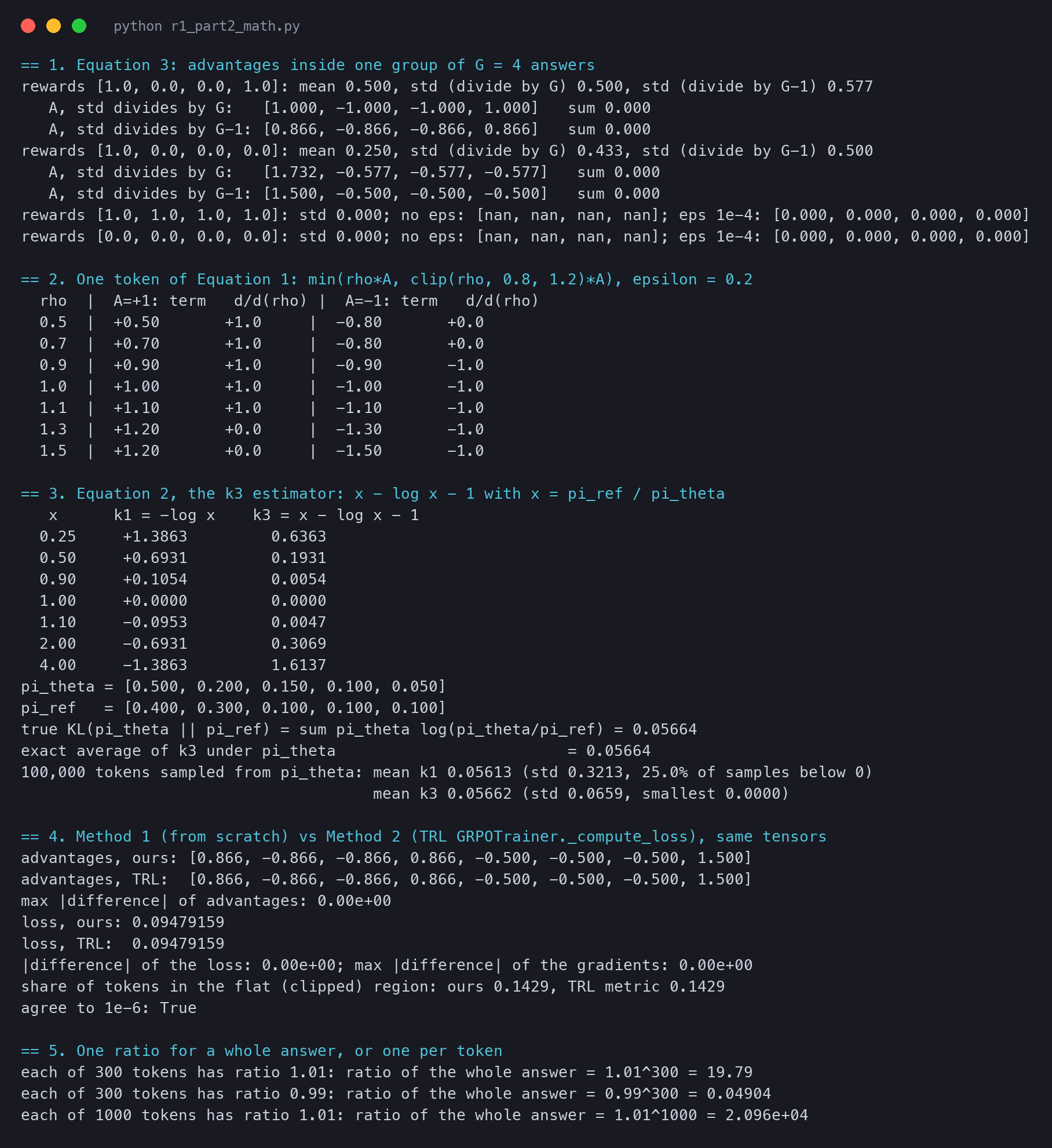
Our script computes the term and its slope (the gradient with respect to ) for a few ratios. A slope of 0 means the token gets no push from this batch.
== 2. One token of Equation 1: min(rho*A, clip(rho, 0.8, 1.2)*A), epsilon = 0.2
  rho  |  A=+1: term   d/d(rho) |  A=-1: term   d/d(rho)
  0.5  |  +0.50       +1.0     |  -0.80       +0.0
  0.7  |  +0.70       +1.0     |  -0.80       +0.0
  0.9  |  +0.90       +1.0     |  -0.90       -1.0
  1.0  |  +1.00       +1.0     |  -1.00       -1.0
  1.1  |  +1.10       +1.0     |  -1.10       -1.0
  1.3  |  +1.20       +0.0     |  -1.30       -1.0
  1.5  |  +1.20       +0.0     |  -1.50       -1.0
Read the left half. For a good answer, ratios below 1.2 keep a slope of +1: keep raising it. At 1.3 and 1.5 the slope is 0: it has risen enough for this batch. Now the right half. For a bad answer at ratio 0.5 or 0.7 the slope is 0: it has already dropped enough. At 1.3 the bad answer became more likely by mistake, and the slope stays at -1, so the error is corrected.
The average over the group: 1/G
averages the answers of one question, so a question counts the same whether is 8 or 64. Inside each answer, the paper's short form hides a second average, over tokens. We come back to it in the per-token section.
The KL penalty: stay near the reference
subtracts a cost for moving away from a reference model. The clip limits one batch. The KL term limits the whole run: after thousands of steps, the model should still be close enough to a sensible starting point. sets how strong that pull is.
The paper's ratio is for a whole answer; code uses tokens
R1's Equation 1 writes , the probability of the whole answer. A language model writes the answer token by token, so this is a product: . The ratio of the whole answer is then the product of the ratios of its tokens.
A product of many numbers near 1 is not near 1. Our script shows it:
== 5. One ratio for a whole answer, or one per token
each of 300 tokens has ratio 1.01: ratio of the whole answer = 1.01^300 = 19.79
each of 300 tokens has ratio 0.99: ratio of the whole answer = 0.99^300 = 0.04904
each of 1000 tokens has ratio 1.01: ratio of the whole answer = 1.01^1000 = 2.096e+04
A change of 1% per token makes the whole-answer ratio 19.79 after 300 tokens. A clip at 1.2 would then stop almost every long answer. R1's answers run to thousands of tokens. So in practice the ratio and the clip apply to each token, and an answer's score is the mean over its tokens. That is DeepSeekMath's Equation 3 with its , which TRL's GRPOTrainer and our code compute. And the R1 paper's short form is best read as notation for this per-token version.
Equation 2: a KL that is never negative
Write for one sampled token. Equation 2 is then .
Why it is never negative. The curve always lies below its tangent line at , which is . So for every , and . The two are equal only at , where the two models agree.
Why its average is the true KL. Average over tokens sampled from . The first part averages to . So the and the cancel on average, and what is left is the average of . That average is exactly the definition of .
Now with numbers. The first table is (the simple estimate) and for a few ratios. Then two small distributions over 5 tokens, the exact KL, and 100,000 sampled tokens:
== 3. Equation 2, the k3 estimator: x - log x - 1 with x = pi_ref / pi_theta
   x      k1 = -log x    k3 = x - log x - 1
  0.25     +1.3863         0.6363
  0.50     +0.6931         0.1931
  0.90     +0.1054         0.0054
  1.00     +0.0000         0.0000
  1.10     -0.0953         0.0047
  2.00     -0.6931         0.3069
  4.00     -1.3863         1.6137
pi_theta = [0.500, 0.200, 0.150, 0.100, 0.050]
pi_ref   = [0.400, 0.300, 0.100, 0.100, 0.100]
true KL(pi_theta || pi_ref) = sum pi_theta log(pi_theta/pi_ref) = 0.05664
exact average of k3 under pi_theta                         = 0.05664
100,000 tokens sampled from pi_theta: mean k1 0.05613 (std 0.3213, 25.0% of samples below 0)
                                      mean k3 0.05662 (std 0.0659, smallest 0.0000)
Check one row by hand. For : . Both estimators average to about the true KL of 0.0566. But a single is below zero for 25% of the sampled tokens. Its spread (0.3213) is also almost five times the spread of (0.0659).
Both are fair on average, so the gain from is not that it is "more right". The gain is a smaller spread for the same average, so fewer samples give a steady estimate.
Note also that "never negative" is a fact about each value, not about its gradient. The gradient is a separate question. One token's has gradient . Averaged over tokens sampled from , that is , the gradient of : the KL with its two sides swapped. Close to the reference the two directions of the KL nearly agree, so in practice the term still keeps the model near the reference.
There is one more choice in Equation 1: the KL goes straight into the loss. PPO for language models usually subtracts a KL penalty from the reward at every token. The later long version of the paper says that in PPO this penalises the cumulative KL, which "may implicitly penalize the length of the response". R1-Zero's answers had to grow long, so a penalty that grows with length would work against it.
Equation 3: the group is the baseline
Four answers, by hand
One question, answers. Answers 1 and 4 are right (reward 1), answers 2 and 3 are wrong (reward 0).
The mean is . Each answer is 0.5 away from the mean, so the standard deviation is 0.5. Then:
The right answers are pushed up, the wrong ones down, with equal force.
There is one detail the paper leaves open: the standard deviation can divide by or by . PyTorch's torch.std and TRL divide by (Bessel's correction), which makes the standard deviation 0.577 here and the advantages . The direction is the same. Only the size changes, by a fixed factor that the learning rate absorbs. Our code uses , like TRL, so the two methods match.
Now a harder question: only answer 1 is right.
rewards [1.0, 0.0, 0.0, 0.0]: mean 0.250, std (divide by G) 0.433, std (divide by G-1) 0.500
   A, std divides by G:   [1.732, -0.577, -0.577, -0.577]   sum 0.000
   A, std divides by G-1: [1.500, -0.500, -0.500, -0.500]   sum 0.000
The one right answer gets a large push (+1.732), and each wrong one a small push down (-0.577). This is the useful part of the rule. A rare success on a hard question is exactly what the model should learn from, and the curve makes it count most. In every case the advantages of a group sum to zero: the group pushes up as much as it pushes down.
When every answer gets the same reward
If all four answers are right, the mean is 1 and every is 0. The standard deviation is also 0, so Equation 3 is . Code needs a small number in the denominator, and TRL adds :
rewards [1.0, 1.0, 1.0, 1.0]: std 0.000; no eps: [nan, nan, nan, nan]; eps 1e-4: [0.000, 0.000, 0.000, 0.000]
rewards [0.0, 0.0, 0.0, 0.0]: std 0.000; no eps: [nan, nan, nan, nan]; eps 1e-4: [0.000, 0.000, 0.000, 0.000]
Without the small number, every advantage is "not a number", and one such value spoils the whole gradient. With it, every advantage is 0, and the reward part of the loss gives no signal for this question. Only the KL term can still move the model, by pulling it toward the reference. In our real run below that term is 0 as well, because the reference is a copy of the current weights.
Giving no reward signal is correct: if all answers are equally good, there is nothing to prefer, but it has a cost. A question that is too easy (all right) or too hard (all wrong) wastes all its samples. GRPO learns only from questions at the edge of what the model can do.
The settings v1 does not give
R1 v1 names and but gives no values, and it does not give . The later long version of the paper (published with the Nature article) does.
GRPO in code, two ways
Method 1: from scratch
Five short functions, one per idea. Shapes are in the comments: is the number of answers in the batch (questions times ) and the longest answer in tokens.
def group_advantages(rewards, G, unbiased=True, eps=1e-4):
    r = rewards.view(-1, G)                                   # (n_questions, G): one row per question
    mean = r.mean(dim=1, keepdim=True)                        # (n_questions, 1): the group's average reward
    std = r.std(dim=1, keepdim=True, unbiased=unbiased)       # (n_questions, 1): the group's spread
    return ((r - mean) / (std + eps)).view(-1)                # (B,): better than the group > 0, worse < 0


def ratio(logp_new, logp_old):
    return torch.exp(logp_new - logp_old)                     # (B, T): pi_theta / pi_theta_old per token


def clipped_surrogate(rho, A, epsilon):
    A = A.unsqueeze(1)                                        # (B, 1): broadcast over the tokens of each answer
    unclipped = rho * A                                       # (B, T): the plain policy-gradient term
    clipped = torch.clamp(rho, 1 - epsilon, 1 + epsilon) * A  # (B, T): the ratio held inside [1 - eps, 1 + eps]
    return torch.minimum(unclipped, clipped)                  # (B, T): the smaller, more careful of the two


def k3_kl(logp_theta, logp_ref):
    log_r = logp_ref - logp_theta                             # (B, T): log of pi_ref / pi_theta
    return torch.exp(log_r) - log_r - 1                       # (B, T): x - log x - 1 >= 0 for every x > 0


def grpo_loss(logp, logp_old, logp_ref, A, mask, epsilon=0.2, beta=0.04):
    rho = ratio(logp, logp_old)                               # (B, T)
    per_token = clipped_surrogate(rho, A, epsilon) - beta * k3_kl(logp, logp_ref)   # (B, T): J per token
    per_answer = (per_token * mask).sum(dim=1) / mask.sum(dim=1).clamp(min=1)       # (B,): 1/|o_i| sum over t
    return -per_answer.mean()                                 # scalar: 1/G sum over i, with a minus to minimise
The last function is Equation 1 with the per-token practice. The mask is 1 on real answer tokens and 0 on padding, because the answers in a batch have different lengths. The minus sign at the end turns "maximise " into "minimise the loss", which is what optimisers do.
Method 2: TRL's GRPOTrainer
TRL is the Hugging Face library for training language models with reinforcement learning. Its GRPOTrainer computes the loss in a method called _compute_loss. Here are its core lines, from trl 1.18 (shortened; the other loss types and the logging are left out):
log_ratio = per_token_logps - old_per_token_logps
coef_1 = torch.exp(log_importance_weights)          # the ratio, per token
per_token_kl = (
    torch.exp(ref_per_token_logps - per_token_logps) - (ref_per_token_logps - per_token_logps) - 1
)                                                   # Equation 2, k3
coef_2 = torch.clamp(coef_1, 1 - self.epsilon_low, 1 + self.epsilon_high)
per_token_loss1 = coef_1 * advantages
per_token_loss2 = coef_2 * advantages
per_token_loss = -torch.min(per_token_loss1, per_token_loss2)
per_token_loss = per_token_loss + self.beta * per_token_kl
loss = ((per_token_loss * mask).sum(-1) / mask.sum(-1).clamp(min=1.0)).mean()   # loss_type="grpo"
It is the same equation, written by other people. We do not copy these lines; we call TRL's real method, which normally runs inside a full trainer with a model and a dataset. Our file r1_part2_trl.py gives it a small stand-in object with only the settings it reads (loss_type='grpo', beta, epsilon). A stand-in model call returns our log-probabilities. Every line of the loss then runs as TRL wrote it.
TRL computes the advantages inside the method that also samples text. So we repeat those lines exactly: a group mean, a group standard deviation with , and .
We feed both methods the same tensors: 2 questions with 4 answers each, 6 tokens per answer with some padding. The log-probabilities of the policy, the old policy and the reference all differ, so the ratios are not 1 and some tokens are clipped.
== 4. Method 1 (from scratch) vs Method 2 (TRL GRPOTrainer._compute_loss), same tensors
advantages, ours: [0.866, -0.866, -0.866, 0.866, -0.500, -0.500, -0.500, 1.500]
advantages, TRL:  [0.866, -0.866, -0.866, 0.866, -0.500, -0.500, -0.500, 1.500]
max |difference| of advantages: 0.00e+00
loss, ours: 0.09479159
loss, TRL:  0.09479159
|difference| of the loss: 0.00e+00; max |difference| of the gradients: 0.00e+00
share of tokens in the flat (clipped) region: ours 0.1429, TRL metric 0.1429
agree to 1e-6: True
The advantages, the loss and the gradients agree to the last bit. In both, 14.29% of the real tokens sit in the flat part of the clip. The first group is our four-answer example (1, 0, 0, 1), with the standard deviation: . The second group has one right answer out of four: +1.5 for it, -0.5 for the others.
One real GRPO step on a small model
Now the same loss on a real model. The script r1_part2_run.py loads Qwen2.5-0.5B-Instruct on a Mac (MPS, float32). For each GSM8K test question, in order, it samples answers at temperature 1, with at most 512 new tokens. A check gives reward 1 when the whole expression in the last \boxed{} equals the reference answer, and 0 otherwise. With no box, it uses the last number in the text.
The check compares the two with math-verify, so a boxed counts as 1.5, not as 3. The script keeps the first question whose group has both right and wrong answers. We use and .
One setting needs care. The model's own configuration file asks for a repetition penalty of 1.1, temperature 0.7, top-p 0.8 and top-k 20 whenever it generates. Each of these changes the probabilities the answers are drawn from. Our loss computes log-probabilities from the plain softmax of the logits. If the two differ, in the ratio is not the policy that really sampled the answers, and the run is no longer on-policy. So the script switches all of them off:
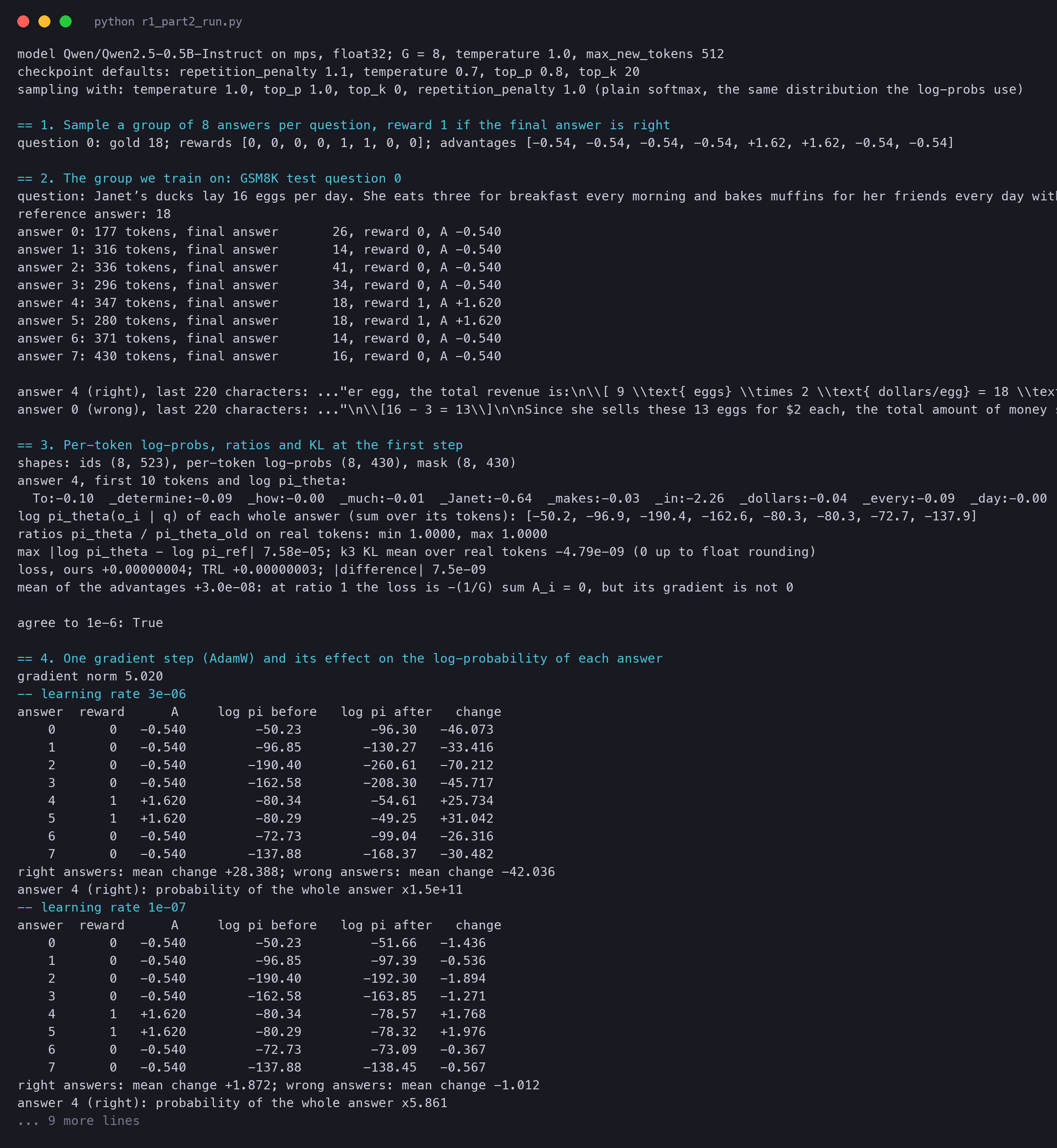
model Qwen/Qwen2.5-0.5B-Instruct on mps, float32; G = 8, temperature 1.0, max_new_tokens 512
checkpoint defaults: repetition_penalty 1.1, temperature 0.7, top_p 0.8, top_k 20
sampling with: temperature 1.0, top_p 1.0, top_k 0, repetition_penalty 1.0 (plain softmax, the same distribution the log-probs use)

== 1. Sample a group of 8 answers per question, reward 1 if the final answer is right
question 0: gold 18; rewards [0, 0, 0, 0, 1, 1, 0, 0]; advantages [-0.54, -0.54, -0.54, -0.54, +1.62, +1.62, -0.54, -0.54]
The very first question already has both right and wrong answers: it is the duck-egg question. Janet's ducks lay 16 eggs a day. She eats 3 for breakfast, bakes muffins with 4, and sells the rest at 2 dollars an egg. How much does she make each day? The answer is , and two of the eight answers get it right.
answer 0: 177 tokens, final answer       26, reward 0, A -0.540
answer 1: 316 tokens, final answer       14, reward 0, A -0.540
answer 2: 336 tokens, final answer       41, reward 0, A -0.540
answer 3: 296 tokens, final answer       34, reward 0, A -0.540
answer 4: 347 tokens, final answer       18, reward 1, A +1.620
answer 5: 280 tokens, final answer       18, reward 1, A +1.620
answer 6: 371 tokens, final answer       14, reward 0, A -0.540
answer 7: 430 tokens, final answer       16, reward 0, A -0.540
Answer 0 is a typical mistake. It subtracts the 3 eggs for breakfast, forgets the 4 for muffins, and sells 13 eggs for 26 dollars.
Check the advantages by hand. The mean reward is . The standard deviation with is . So each right answer gets and each wrong one . The two pushes up balance the six pushes down: .
Log-probabilities, ratios and the loss at the first step
== 3. Per-token log-probs, ratios and KL at the first step
shapes: ids (8, 523), per-token log-probs (8, 430), mask (8, 430)
answer 4, first 10 tokens and log pi_theta:
  To:-0.10  _determine:-0.09  _how:-0.00  _much:-0.01  _Janet:-0.64  _makes:-0.03  _in:-2.26  _dollars:-0.04  _every:-0.09  _day:-0.00
log pi_theta(o_i | q) of each whole answer (sum over its tokens): [-50.2, -96.9, -190.4, -162.6, -80.3, -80.3, -72.7, -137.9]
ratios pi_theta / pi_theta_old on real tokens: min 1.0000, max 1.0000
max |log pi_theta - log pi_ref| 7.58e-05; k3 KL mean over real tokens -4.79e-09 (0 up to float rounding)
loss, ours +0.00000004; TRL +0.00000003; |difference| 7.5e-09
mean of the advantages +3.0e-08: at ratio 1 the loss is -(1/G) sum A_i = 0, but its gradient is not 0
The batch is 8 rows of 523 tokens: the prompt, then up to 430 answer tokens. The mask marks the real answer tokens. Each token has a log-probability: "To" at the start of answer 4 has , so the model gave it probability . Summed over the 347 tokens of answer 4, the log-probability of the whole answer is .
Every ratio is exactly 1.0000. The old policy is the model that just sampled, and no step has happened yet, so . TRL does the same: with one update per batch, it reuses the current log-probabilities, detached, as the old ones.
In this toy run the reference is also a copy of the same weights. A second forward pass on the GPU differs only by of rounding, so the KL term is 0 too. In real training, after many steps, the reference would differ and the KL term would not be 0. As predicted, the loss is 0 (up to rounding) in both methods, and they agree to .
One gradient step
The gradient of that zero loss has a norm of 5.020. We take one AdamW step from the same weights twice: once with the later version's learning rate, , and once with .
-- learning rate 3e-06
right answers: mean change +28.388; wrong answers: mean change -42.036
answer 4 (right): probability of the whole answer x1.5e+11
-- learning rate 1e-07
answer  reward      A     log pi before   log pi after   change
    0       0   -0.540         -50.23         -51.66   -1.436
    1       0   -0.540         -96.85         -97.39   -0.536
    2       0   -0.540        -190.40        -192.30   -1.894
    3       0   -0.540        -162.58        -163.85   -1.271
    4       1   +1.620         -80.34         -78.57   +1.768
    5       1   +1.620         -80.29         -78.32   +1.976
    6       0   -0.540         -72.73         -73.09   -0.367
    7       0   -0.540        -137.88        -138.45   -0.567
right answers: mean change +1.872; wrong answers: mean change -1.012
answer 4 (right): probability of the whole answer x5.861
The direction is right at both sizes: both right answers go up and all six wrong ones go down. The size needs care. Adam's first step moves every weight by about the learning rate, whatever the size of its gradient. Over 494 million weights that adds up. With on one tiny batch, right answer 4 became times more likely, a huge jump.
In real training a step averages over 512 answers, and Adam's statistics settle over many steps. So for a readable picture we keep . Right answer 4 becomes 5.861 times more likely, and the wrong answers lose about 1 in log-probability on average.
The second step: the ratios and the clip wake up
== 5. The same batch after the step with learning rate 1e-07: ratios move away from 1
per-token ratios: min 0.6318, max 1.2368, outside [0.8, 1.2]: 0.12% of 2553 tokens
answer 4: whole-answer ratio exp(sum of log ratios) = 5.861
k3 KL to the reference, mean over real tokens: 2.10e-04
loss at the second step, ours -0.00387105; TRL -0.00387105; |difference| 0.0e+00
share of tokens in the flat (clipped) region, TRL metric: 0.12%
(the loss went from +0.000000 to -0.003871)
If we trained a second time on the same batch, as R1 does with its 16 mini-batches, the ratios would no longer be 1. Per token they now run from 0.632 to 1.237, and 0.12% of the 2,553 real tokens are outside . The ratio of the whole of answer 4 is 5.861, far outside any clip. That is the per-token point in practice: each token moved a little, and the whole answer moved a lot. The KL to the reference is no longer 0 but small, per token. The loss went down from 0 to , and our code and TRL print the same value to every digit shown (difference 0.0e+00).
This is one step on one question. Part 8 runs the loop for many steps and trains a small model to reason. First, Part 3 looks at where the rewards come from.
The paper and the code
Paper (arXiv 2501.12948) · Official repository · Our scripts for this series