vLLM, explained · Part 5 of 6 · Covers §6 to §10, Figures 11 to 19
The Experiments
How the paper tests vLLM against FasterTransformer and three versions of Orca, how to read its latency plots, and what the ablations show. We rebuild the main experiments as a small serving simulation on real request lengths.
Efficient Memory Management for Large Language Model Serving with PagedAttention. Woosuk Kwon, Zhuohan Li, Siyuan Zhuang, Ying Sheng, Lianmin Zheng, Cody Hao Yu, Joseph E. Gonzalez, Hao Zhang, Ion Stoica. SOSP 2023, 2023. arXiv:2309.06180
Parts 1 to 4 built the idea. Store each request's KV cache in small blocks, hand them out on demand, and share them when requests can. This part asks the question that decides whether any of it matters. On a real GPU with real requests, does vLLM serve more people at the same speed?
Each piece below shows the exact lines of the paper, then explains them. Next to the paper's numbers we put our own: a small serving simulator fed with real request lengths. Those numbers come from a laptop, not from the paper's A100 GPUs, and the page says so each time.
Parts 3 and 4 opened the boxes of vLLM one by one. This part closes them again. It treats the whole system as one machine: requests go in on the left, answers come out, and a stopwatch measures each request. The map below is the paper's Figure 4, redrawn. The highlighted scheduler, with its KV cache manager, is the piece that changes from one system to the next.
The vLLM architecture, redrawn from the paper's Figure 4 as a map. Part 5 measures it from the outside. Each baseline keeps the workers and the model, and replaces the highlighted scheduler and memory manager with its own.
Before we read the paper's tests, we need the shape of any serving test. It is the same for a web server, a database or a language model.
A serving test has three inputs. The first is the requests: for us, a prompt length and an answer length each. The second is the arrival times: when each request reaches the server. The third is the server itself, the system under test. The test keeps the first two fixed and swaps the third.
The test then reads two kinds of numbers. One is how much work the server finishes per second. The other is how long each user waits. The next two boxes name them.
A good server has both: high throughput and low latency. The two pull against each other. A server can raise its throughput by packing more requests into each step, but each request then waits longer. So the paper does not report one number. It reports a curve: latency at each request rate.
Table 1 is a division: the memory for the KV cache over the size of one slot, from Part 2. A tiny case first. If one slot were 1 MB and the cache had 10 MB, there would be 10 slots. We check the real table with the real model configurations. The function gives the bytes of one slot; look at the last two columns of the output, ours and the paper's:
python
def kv_bytes_per_token(layers, hidden, bytes_per_value=2):
    """A key and a value (2) of `hidden` numbers in every layer, 2 bytes each in FP16."""
    return 2 * layers * hidden * bytes_per_value
plain text
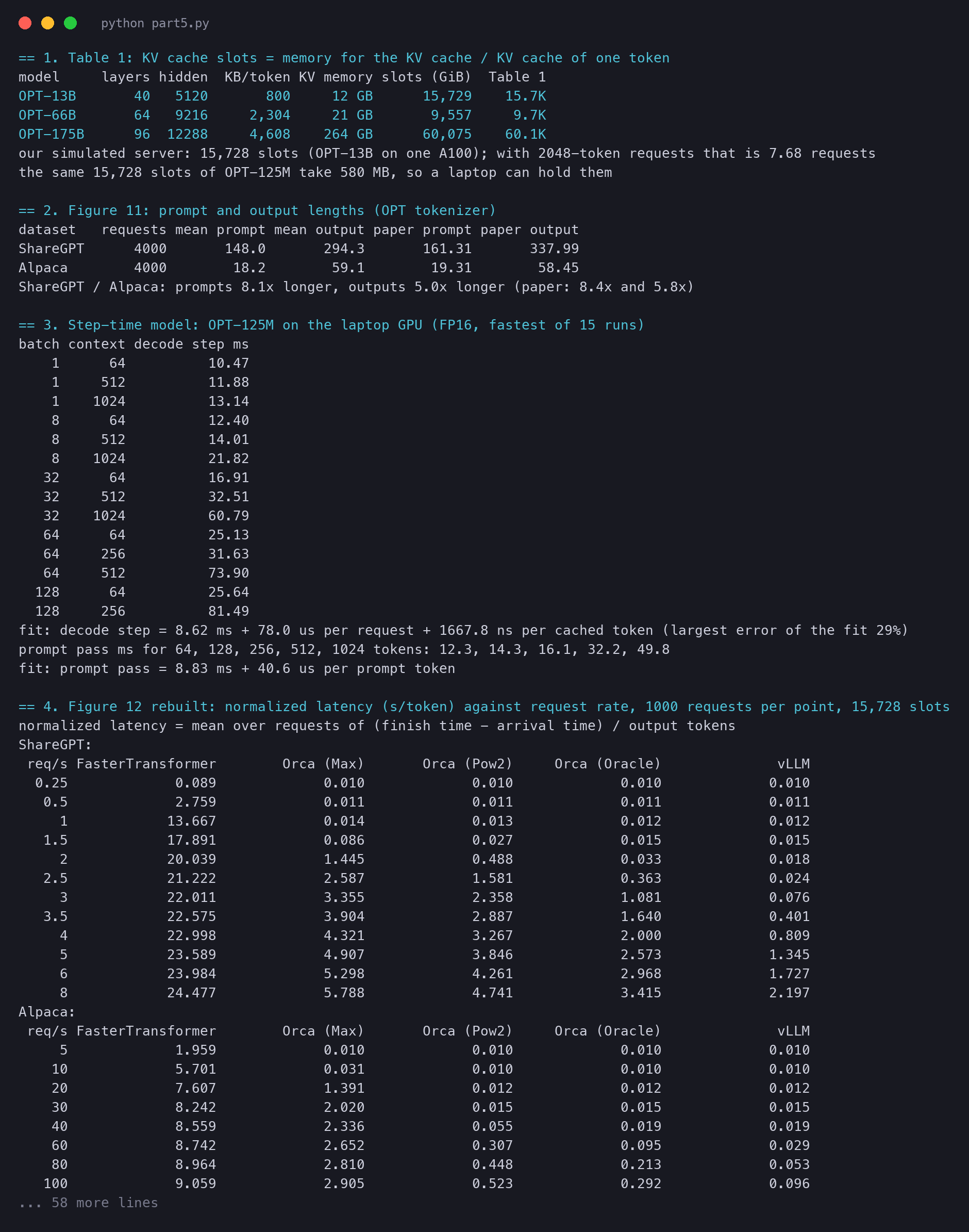
== 1. Table 1: KV cache slots = memory for the KV cache / KV cache of one tokenmodel layers hidden KB/token KV memory slots (GiB) Table 1OPT-13B 40 5120 800 12 GB 15,729 15.7KOPT-66B 64 9216 2,304 21 GB 9,557 9.7KOPT-175B 96 12288 4,608 264 GB 60,075 60.1Kour simulated server: 15,728 slots (OPT-13B on one A100); with 2048-token requests that is 7.68 requeststhe same 15,728 slots of OPT-125M take 580 MB, so a laptop can hold them
Two rows match exactly once we read "GB" as binary gigabytes (GiB, 230 bytes). For OPT-66B we get 9,557 slots, a little under the table's 9.7K; the table probably rounds the memory. The first row is our server for the rest of this part: 15,728 slots. Only 7.68 requests of the full 2,048 tokens fit in it. Remember that number.
The picture shows the difference. Both rows have the same average rate of 1 request per second. The top row is a metronome. The bottom row is one random draw of Poisson arrivals, from the same generator our simulator uses.
Regular arrivals against Poisson arrivals at the same average rate. The random row has clumps, three requests in less than a tenth of a second, and long quiet gaps. A server must absorb the clumps, so random arrivals are harder to serve than regular ones.
We repeat the counting on 4,000 requests of each dataset, with the OPT tokenizer. For ShareGPT we take the first question and its answer. The paper does not say exactly how it cut the conversations, so our ShareGPT numbers cannot match to the token:
plain text
== 2. Figure 11: prompt and output lengths (OPT tokenizer)dataset requests mean prompt mean output paper prompt paper outputShareGPT 4000 148.0 294.3 161.31 337.99Alpaca 4000 18.2 59.1 19.31 58.45ShareGPT / Alpaca: prompts 8.1x longer, outputs 5.0x longer (paper: 8.4x and 5.8x)
Our requests, counted with the OPT tokenizer. ShareGPT prompts and answers spread out to 2,000 tokens; Alpaca is packed near zero. Compare with the paper's Figure 11 above.
Alpaca matches closely: 18.2 and 59.1 tokens against the paper's 19.31 and 58.45. ShareGPT is near too, with 8.1 times longer prompts against the paper's 8.4. Note the long tail of ShareGPT answers: the unknown length of Part 2, now with real data.
The arrival times come from a few lines of code. Each gap is drawn from an exponential distribution with a mean of one over the rate. At 2 requests per second, the mean gap is half a second. The function adds the gaps one by one to get the arrival times:
python
def poisson(n, rate, seed):
    """Arrival times of n requests: gaps drawn from an exponential distribution with mean 1 / rate."""
    r, t, out = random.Random(seed), 0.0, []
    for _ in range(n):
        t += r.expovariate(rate); out.append(t)
    return out
A baseline is the system you compare against. A new system is only as good as the strongest baseline it beats. The paper picks two families: the fastest engine of the day, and the best scheduler of the day.
The three Orca versions differ only in how much answer they book. Max books for the worst case, Pow2 books up to twice the real answer, and Oracle books the real answer. In our simulator, this function gives the slots each version books for a prompt of p tokens and an answer of o tokens. Then our buddy allocator rounds that up to a power of two:
python
def reserve(system, p, o):
    """Slots that an Orca version books for a request at admission (before the buddy allocator rounds it up)."""
    if system == 'Orca (Max)':
        return 2048                                            # the model's maximum sequence length
    if system == 'Orca (Pow2)':
        return p + (1 << (o - 1).bit_length())                 # output booked up to 2x: 25 -> 32
    return p + o                                               # Oracle: knows the real output length
A worked example. A request has a prompt of 19 tokens and an answer of 25. Oracle books 19+25=44 slots, and the buddy allocator gives it 64. Pow2 books 19+32=51, which also becomes 64. Max books 2,048.
With 16-token blocks, vLLM holds 2 blocks (32 slots) right after the prompt. At the end, after all 44 tokens, it holds 3 blocks (48 slots).
One request, five systems. Blue is the prompt, orange is the answer that the model really writes, and the dashed red part is memory set aside but never used. Only vLLM keeps the waste below one block.
The picture is the whole experiment in small. Every system writes the same 44 tokens. FasterTransformer and Orca (Max) block 2,048 slots to do it, about 46 times more than needed. Even the perfect guess of Oracle loses 20 slots to the buddy rounding. The vLLM bar loses 4, and it takes its blocks one at a time, as the answer grows.
In symbols, with N requests, arrival times ai, finish times fi and output lengths oi:
normalized latency=N1i=1∑Noifi−ai
Read it from left to right. It is an average over the N requests. Each term is fi−ai, the time request i spent waiting plus running, divided by its oi answer tokens.
A tiny example with three requests, small enough to check by hand:
request
arrives
finishes
answer tokens
(finish - arrive) / tokens
A
0 s
2 s
100
2 / 100 = 0.02
B
1 s
5 s
50
4 / 50 = 0.08
C
1.5 s
3.5 s
10
2 / 10 = 0.20
The mean is (0.02+0.08+0.20)/3=0.10 s/token. Request B waited in a queue, and its number is four times that of A. Request C wrote only 10 tokens, so each of its seconds weighs heavily. The short requests count as much as the long ones in the mean.
The paper says it focuses on throughput, but it plots latency. The two are linked. The throughput of a server, in the paper's sense, is the highest request rate it can take while the normalized latency stays low. A user never sees throughput. A user sees the wait for each token.
We cannot run OPT-13B on an A100 here. We can rebuild the experiment's logic and keep the part that the paper is about: memory. Our simulator has five pieces.
Requests: 1,000 real (prompt, answer) lengths from ShareGPT or Alpaca, with Poisson arrival times.
Memory: 15,728 slots, the Table 1 budget of OPT-13B on one A100.
Five ways to store the cache: FasterTransformer, three Orca versions with a real buddy allocator, and vLLM. Its 16-token blocks come with preemption by recomputation (Part 4, and the box below).
A scheduler: first come, first served, at most 256 running requests, as in vLLM's default setting.
A clock: each iteration costs a time from a step-time model measured on our laptop.
A step with more requests, or with longer caches, takes longer. We time real decode steps of OPT-125M on the laptop GPU for many batch sizes and cache lengths, and fit a straight line:
python
def step_time(n_decode, cached, prompt_tokens):
    """One iteration: the fixed cost, plus each decoding request, plus each cached token it reads, plus prompt tokens."""
    return A_STEP + B_REQ * n_decode + C_TOK * cached + E_PRE * prompt_tokens
plain text
== 3. Step-time model: OPT-125M on the laptop GPU (FP16, fastest of 15 runs)batch context decode step ms 1 64 10.47 1 512 11.88 1 1024 13.14 8 64 12.40 8 512 14.01 8 1024 21.82 32 64 16.91 32 512 32.51 32 1024 60.79 64 64 25.13 64 256 31.63 64 512 73.90 128 64 25.64 128 256 81.49fit: decode step = 8.62 ms + 78.0 us per request + 1667.8 ns per cached token (largest error of the fit 29%)prompt pass ms for 64, 128, 256, 512, 1024 tokens: 12.3, 14.3, 16.1, 32.2, 49.8fit: prompt pass = 8.83 ms + 40.6 us per prompt token
One decode step costs 8.62 ms even for a single request: the fixed cost of a pass through the model, which batching shares. Each cached token adds about 1.7 microseconds, because attention must read it. The fit is off by up to 29%, and the laptop was busy with other work. So treat our seconds as a shape, not as a server measurement.
The heart of the simulator is the vLLM path. Before each iteration, every running request needs room for one more token. If a new block is needed and none is free, the latest arrival gives up all its blocks. It goes back to the front of the queue.
A small case shows the rule. Say 2 blocks are free, and three running requests each need a new block. The first two get them. The third finds none, so the request that arrived last is preempted, and its blocks pay for the third. In the code, need is the number of new blocks a request needs, free the free blocks, and hold the blocks each request holds:
python
        if paged:                                              # room for one more token in each running request
            k = 0
            while k < len(running):
                i = running[k]
                need = -(-(P[i] + gen[i] + 1) // block) - hold[i]
                while need > free and running[-1] != i:        # preempt the latest arrival: free all its blocks
                    v = running.pop(); free += hold.pop(v); waiting.appendleft(v); preempt += 1; preempted = True
                if need > free:                                # i itself is the latest arrival
                    running.pop(); free += hold.pop(i); waiting.appendleft(i); preempt += 1; preempted = True
                    break
                free -= need; hold[i] += need; k += 1
The expression -(-x // block) is the number of blocks that x tokens need, rounded up. For 17 tokens and blocks of 16, it gives 2. In the Orca path there is no such loop. A request joins only if the buddy allocator finds a chunk for its whole reservation, and it never needs more.
The paper's main figures all have the same shape, so it pays to learn to read one first. The picture below is drawn on our own ShareGPT run, with only two systems. Read the four numbered marks in order.
Anatomy of a latency plot. (1) At low load every system sits on the same flat floor. (2) At the knee the batch is full and a queue starts. (3) Past the knee the line becomes a wall. (4) The system whose knee is further right serves more users on the same GPU.
The horizontal axis is the load: requests per second. The vertical axis is the normalized latency: how slow each token feels to a user. A point on a line answers one question. If users arrive at this rate, how slow does this system feel?
On the floor, the server has spare room. Each request is served at once, and the latency is just the time to compute a token. At the knee, the batch is as large as memory allows, and newcomers start to wait. The wall follows: the queue grows, and so does every wait. So the plot is not about the height of the lines. It is about where each line leaves the floor.
The simplest queue has one cashier and random arrivals. Customers arrive at a rate λ (lambda) per minute, and the cashier serves μ (mu) per minute on average, also at random. Queueing theory gives the mean time a customer spends in the shop, queue and checkout together:
W=μ−λ1
Read it from left to right. W is the mean time in the shop. The bottom, μ−λ, is the spare speed of the cashier: how many more customers a minute it could serve. The formula holds only while λ<μ.
A worked example with a cashier who serves μ=10 customers a minute. At λ=5, W=1/5 of a minute, or 12 seconds. At λ=8, W=1/2 minute, 30 seconds. At λ=9, W=1 minute. At λ=9.9, W=10 minutes. The last 10% of load costs far more than the first 90%.
The cashier's queue from the formula above. The mean time in the shop stays low up to about half the cashier's speed, then climbs ever faster, and has no limit at 10 customers a minute. It is the same shape as each line in Figure 12.
A language model server is not a single cashier. It serves a whole batch at once, and its speed changes with the batch. But the shape carries over. Its "cashier speed" is the rate at which its memory lets requests through. vLLM raises that speed, because more requests fit in memory. So its wall moves to the right.
Here is our simulator on the same experiment. Each point is a run of 1,000 requests. We use OPT-125M step times and the 15,728 slots of OPT-13B. Each row is one request rate, and each column one system. Read down a column: the number stays near 0.01, then jumps. Look at which column jumps first:
Our simulation of Figure 12, cut at 1.0 s/token as in the paper. The order of the bends is the paper's order: FasterTransformer, then Orca (Max), Orca (Pow2), Orca (Oracle) and vLLM. FasterTransformer on Alpaca is above 1.0 s/token even at 5 requests per second, so its line is off the chart.
At low load, all four iteration-level systems give the same 0.010 s/token on ShareGPT: when nobody waits, memory management does not matter. Then the bends appear in the paper's order. To turn bends into "times higher", we draw a line at 0.1 s/token, about ten times the unloaded latency. Then we read where each curve crosses it:
python
def crossing(rates, vals, limit=LIMIT):
    """The rate at which the curve first rises above the limit, read between the two points around it."""
    if vals[0] > limit:
        return 0.0
    for (r0, v0), (r1, v1) in zip(zip(rates, vals), zip(rates[1:], vals[1:])):
        if v1 > limit:
            return r0 + (r1 - r0) * (limit - v0) / (v1 - v0)
    return float('inf')
plain text
request rate where normalized latency crosses 0.1 s/token (our "same latency" line, linear between points):ShareGPT FasterTransformer 0.3, Orca (Max) 1.5, Orca (Pow2) 1.6, Orca (Oracle) 2.1, vLLM 3.0 vLLM / Orca (Oracle) = 1.4x, vLLM / Orca (Pow2) = 1.9x, vLLM / Orca (Max) = 2.0xAlpaca FasterTransformer < 5, Orca (Max) 10.5, Orca (Pow2) 43.6, Orca (Oracle) 60.8, vLLM 102.3 vLLM / Orca (Oracle) = 1.7x, vLLM / Orca (Pow2) = 2.3x, vLLM / Orca (Max) = 9.7xpaper, ShareGPT: vLLM sustains 1.7x to 2.7x the rate of Orca (Oracle), 2.7x to 8x that of Orca (Max), up to 22x that of FasterTransformer
How to read "times higher". Fix a latency (the dashed line), find where each curve crosses it, and divide the two rates. On our ShareGPT run, Orca (Oracle) crosses at 2.1 requests per second and vLLM at 3.0.
The choice of 0.1 s/token is ours; the paper does not give the latency level it used. Another line would give other ratios, but in our table the order of the systems is the same at every rate.
Our simulator gives the same bars. We let all 1,000 requests arrive at time 0, so the queue is never empty, and we count the running requests at each iteration. We also check the count with a second method. When memory is full, the slots held by the running requests add up to the budget. A request stays in the batch for o steps, so a running request is a long request more often than a short one. That gives a closed form:
batch≈S⋅∑i∑g=1oimi(g)∑ioi
Read it from left to right. S is the budget, 15,728 slots. The top sum adds up the answer lengths, so it counts request-steps. The bottom sum adds up mi(g), the slots that request i holds after writing g tokens, over its whole life.
The fraction is one over the slots of an average running request. For Orca, mi(g) is its buddy chunk at every step; for vLLM, the blocks it holds so far.
A tiny example. Two requests, with answers of 1 and 3 tokens. Each holds 4 slots at every step. The sums are 1+3=4 request-steps and 4⋅1+4⋅3=16 slot-steps, so a running request holds 4 slots on average. With S=40, the batch is 40⋅4/16=10.
python
def closed_form_batch(system, reqs, block=16, slots=S):
    """Method 2: when memory is full, the slots held by the running requests add up to the budget. A request is
    running for o steps, so a random running request is picked in proportion to o. Fragmentation is ignored."""
    held = 0
    for p, o in reqs:
        if system == 'vLLM':
            held += sum(block * -(-(p + g) // block) for g in range(1, o + 1))   # blocks grow as it writes
        else:
            held += o * (1 << (reserve(system, p, o) - 1).bit_length())         # one chunk for its whole life
    return slots * sum(o for _, o in reqs) / held
plain text
== 5. Figure 13 rebuilt: requests running at once while the queue is never empty (all arrive at time 0)ShareGPT: system simulated closed form tokens/step tokens/s preemptions Orca (Max) 7.00 7.68 6.9 495 0 Orca (Pow2) 9.30 10.55 9.1 583 0 Orca (Oracle) 14.91 17.08 14.5 731 0 vLLM 37.54 38.02 34.8 952 1443 vLLM against Orca (Oracle): 2.4x the tokens per step, 1.3x the tokens per second (bigger batches make each step slower) vLLM runs 2.5x the requests of Orca (Oracle) and 5.4x those of Orca (Max)Alpaca: system simulated closed form tokens/step tokens/s preemptions Orca (Max) 7.00 7.68 6.9 678 0 Orca (Pow2) 43.98 46.55 36.6 2,211 0 Orca (Oracle) 75.91 82.34 57.3 2,723 0 vLLM 204.01 183.95 103.9 3,296 274 vLLM against Orca (Oracle): 1.8x the tokens per step, 1.2x the tokens per second (bigger batches make each step slower) vLLM runs 2.7x the requests of Orca (Oracle) and 29.1x those of Orca (Max)paper, Figure 13 (OPT-13B, A100): ShareGPT 7.00, 9.81, 13.62, 30.42; Alpaca 7.00, 43.24, 72.75, 132.44note: we cap a batch at 256 requests, as vLLM did by default
Requests in the batch, our simulation next to the paper's Figure 13. The Orca bars are close to the paper's on both datasets. Our vLLM bars are higher than the paper's, most of all on Alpaca.
Orca (Max) gives exactly 7.00, as in the paper. The closed form says 7.68, and the gap is the buddy allocator. The budget of 15,728 is not a power of two, so it is split into pieces of 8,192, 4,096 and fewer slots. Only seven chunks of 2,048 fit in them. That lost 0.68 of a request is external fragmentation: free memory cut into pieces too small to use. It appears on its own.
For Orca (Pow2) and Orca (Oracle), the simulation sits 5% to 13% below the closed form: chunks of mixed sizes leave holes. For vLLM on ShareGPT, the two methods agree within 1.3%, because equal blocks leave no holes. On Alpaca, the 256-request cap and the 274 preemptions break the formula's assumption of a steady, full memory.
Our Orca bars are close to the paper's: 9.30 against 9.81, 14.91 against 13.62, 43.98 against 43.24, 75.91 against 72.75. Memory counts depend only on lengths and budget, so a laptop can get them right. Our vLLM bars are higher, 37.54 against 30.42 and 204 against 132, because a real server has limits that we leave out.
The picture below puts the ShareGPT bars into memory. Each bar is the same 15,728 slots. It is cut into one piece per running request, and the blue part of each piece is what an average running request really holds.
Before vLLM and with vLLM, on the same memory. Orca (Max) cuts it into 7 chunks of 2,048 slots, mostly empty, and 1,392 slots are left over, too small for an eighth chunk. Orca (Oracle) fits about 15 requests, with empty room and holes in each. vLLM fills the memory with about 37 requests.
The blue part is the same size in all three bars: about 419 slots, or 15,728 divided by vLLM's 37.54 requests. That is fair, because a running request holds the same tokens whatever system serves it. Only the empty part around it changes. Remove the empty part, and the same memory holds 5.4 times as many requests as Orca (Max).
Now the reason our speed gains are smaller. On ShareGPT, vLLM writes 2.4 times as many tokens per step as Orca (Oracle), but only 1.3 times as many per second. On our laptop, a step with 38 requests and their caches takes much longer than a step with 15. On an A100, each step must read 26 GB of weights, a fixed cost that a bigger batch shares. The next box shows what happens when that stops being true.
We rebuild the parallel sampling bars two ways. Method 1 is a small block manager with reference counts and copy-on-write, as in Part 4. Method 2 is a closed form. After the first step, only the ⌊p/16⌋ full prompt blocks stay shared, so with n samples and ℓ=p+g tokens each:
blocks without sharing=n⌈16ℓ⌉,blocks with sharing=⌊16p⌋+n(⌈16ℓ⌉−⌊16p⌋)
Read it this way. ⌈ℓ/16⌉ is the blocks one sample needs for ℓ tokens, rounded up. Without sharing, each of the n samples has all of them. With sharing, the full prompt blocks are stored once, and each sample keeps only its own blocks after them.
A tiny example: p=18, two samples, each with 6 new tokens, so ℓ=24. Without sharing, 2⋅2=4 blocks. With sharing, 1+2⋅(2−1)=3 blocks. That saves 1 block of 4, or 25%, at this step.
python
def sharing_refcount(p, o, n, block=16):
    """Method 1: a block manager. The prompt blocks are mapped by all n samples (reference count n). When a sample
    writes into a block that others still map, it gets its own copy first (copy-on-write). Each step we count the
    physical blocks in use and the blocks that n separate copies would need."""
    ref, nxt = {}, 0

    def new_block():
        nonlocal nxt
        ref[nxt] = 1; nxt += 1
        return nxt - 1
    prompt_blocks = [new_block() for _ in range(-(-p // block))]
    for b in prompt_blocks:
        ref[b] = n
    tables, length = [list(prompt_blocks) for _ in range(n)], [p] * n
    with_sharing = without = 0
    for _ in range(o):                                         # each step, every sample writes one token
        for s in range(n):
            if length[s] % block == 0:
                tables[s].append(new_block())                 # the last block is full: take a fresh one
            elif ref[tables[s][-1]] > 1:                       # shared and about to change: copy-on-write
                ref[tables[s][-1]] -= 1; tables[s][-1] = new_block()
            length[s] += 1
        with_sharing += sum(1 for c in ref.values() if c > 0)
        without += sum(len(t) for t in tables)
    return with_sharing, without
plain text
== 6. Figure 15a rebuilt: memory saved by sharing prompt blocks in parallel sampling (block size 16)ShareGPT 2 samples: saved 20.74% (block manager), 20.74% (closed form)ShareGPT 4 samples: saved 31.10% (block manager), 31.10% (closed form)ShareGPT 6 samples: saved 34.56% (block manager), 34.56% (closed form)Alpaca 2 samples: saved 4.51% (block manager), 4.51% (closed form)Alpaca 4 samples: saved 6.76% (block manager), 6.76% (closed form)Alpaca 6 samples: saved 7.52% (block manager), 7.52% (closed form)paper, Figure 15a (Alpaca): 6.09%, 8.53%, 9.79%; §6.3 (ShareGPT): 16.2% to 30.5%assumption: all samples of a request write as many tokens as the dataset answer (real samples differ)
The block manager and the formula agree to every digit. Our Alpaca savings, 4.51% to 7.52%, are a little under the paper's 6.09% to 9.79%. Our ShareGPT savings, 20.74% to 34.56%, are a little over its 16.2% to 30.5%. The pattern is the same: more samples save more, with diminishing returns, and long prompts save far more. One assumption shapes our numbers: every sample writes as many tokens as the dataset's answer, while real samples stop at different times. We did not rebuild beam search, whose sharing depends on the model's choices.
An ablation test removes or changes one part of a system to see what that part contributes. Section 7 asks what vLLM's design costs and which settings are right.
Our simulator can show only one side of this tug of war. It counts memory exactly, but its step time does not depend on the block size, so tiny blocks cost nothing in it. We run vLLM with block sizes 1 to 256, at the rate where 16-token blocks reach our 0.1 s/token line:
plain text
== 7. Figure 18b rebuilt: vLLM in the simulator with block sizes 1 to 256 (memory only, no kernel cost)ShareGPT at 3.0 req/s: 1: 0.072, 2: 0.073, 4: 0.072, 8: 0.074, 16: 0.076, 32: 0.080, 64: 0.085, 128: 0.107, 256: 0.150Alpaca at 102.3 req/s: 1: 0.084, 2: 0.085, 4: 0.086, 8: 0.092, 16: 0.100, 32: 0.114, 64: 0.148, 128: 0.221, 256: 0.392
Our simulator with block sizes 1 to 256. Without a kernel cost, small blocks are free, so only the right side of the paper's Figure 18b appears: large blocks hurt, and they hurt short Alpaca requests far more.
The right side of the paper's figure appears clearly. From 16 to 256, Alpaca's latency grows almost four times, from 0.100 to 0.392 s/token. ShareGPT's grows by about half, from 0.076 to 0.150. Short requests suffer more from large blocks, as the paper says.
The left side does not appear, and that is the lesson. In our simulator, block size 1 is the best. The paper's high latency at block sizes 1 to 4 comes from the GPU kernel, which we did not model. So memory alone pushes toward small blocks, and the GPU kernel sets the lower limit.
We time both on the laptop. We take the real KV cache of OPT-125M after a 1,024-token prompt. We copy it to CPU memory and back, one block of each layer at a time, for block sizes 1 to 256. Then we time one prompt pass that rebuilds the same cache:
python
for b in BS:
    def out():
        for g, c in zip(gpu, cpu):
            for j in range(0, CTX, b):
                c[:, :, j:j + b].copy_(g[:, :, j:j + b])

    def back():
        for g, c in zip(gpu, cpu):
            for j in range(0, CTX, b):
                g[:, :, j:j + b].copy_(c[:, :, j:j + b])
    t_out, t_in = fastest(out, 3), fastest(back, 3)
plain text
== 8. Figure 19a rebuilt: move a 1,024-token KV cache (OPT-125M, FP16) GPU -> CPU -> GPU, block by block, against recomputing it with one prompt pass (laptop, fastest of 3 runs)KV cache: 37.7 MB in 24 tensors; recompute (one prompt pass): 21.1 msblock copies swap out ms swap in ms 1 24,576 7350.2 5298.7 2 12,288 2826.4 2787.9 4 6,144 1278.6 1217.5 8 3,072 716.2 577.4 16 1,536 351.9 325.7 32 768 131.6 165.3 64 384 126.7 151.3 128 192 56.5 56.4 256 96 29.2 29.4swap in + out against recompute: 599x slower at block size 1, 2.8x at block size 256; never faster on this laptop
Our laptop version of Figure 19a, on a log scale. Swapping gets cheaper as blocks grow, because there are fewer copies. Recomputing does not depend on the block size at all.
The shape is the paper's. With 1-token blocks, the cache becomes 24,576 copies: 7,350 ms to move it out and 5,299 ms to move it back. With 256-token blocks it is 96 copies, 29.2 ms out and 29.4 ms back. The start-up cost of each copy dominates. Recomputation takes 21.1 ms at every block size.
The ending differs. On the A100, swapping wins at large blocks. On our laptop, recomputation wins at every size, by 2.8 times even at 256. An Apple laptop has no PCIe link, each small copy is a separate GPU command, and a 125M model recomputes 1,024 tokens very quickly. So the winner depends on the hardware, which is why vLLM supports both.
Some limits are the paper's. Orca was not public, so the authors rebuilt it with an assumed buddy allocator. The largest numbers, 8× and 22×, compare against Orca (Max) and FasterTransformer; against the best possible Orca the ShareGPT gain is 1.7× to 2.7×. Arrival times are random, while real traffic comes in bursts. And the gain shrinks when memory is not the limit, as Figure 12 (f) and §8 say.
Some limits are ours. The simulator is a model, not vLLM. Its clock comes from OPT-125M on a busy laptop, with a fit that is off by up to 29%. It also leaves out some limits of a real server. On our laptop a larger batch makes each step much slower than on an A100, so our speed gains are smaller than the paper's. What our runs show reliably is the memory side: how many requests fit, and why.
Next, in Part 6: build it from scratch. A small paged KV cache and serving loop in Python, checked against a library model.
Run it yourself
The script behind this part is code/papers/vllm/vllm_part5.py. It checks Table 1 and counts the lengths of ShareGPT and Alpaca requests. It times OPT-125M steps on the laptop GPU and fits a step-time model. Then it runs the serving simulator for five systems and checks its batch sizes with a closed form.
Last, it counts the blocks of parallel sampling two ways, sweeps the block size, and times swapping against recomputing. Every number is saved in results/part5.json. On an Apple M-series laptop it takes a few minutes after the downloads. The timings change from run to run.
bash
pip install torch transformers datasets numpypython vllm_part5.py # downloads facebook/opt-125m, two OPT configs, tatsu-lab/alpaca and the ShareGPT file (about 670 MB)
The first 60 lines of the output of vllm_part5.py, as it ran for this article. The full log is results/part5_stdout.txt.