How a language model writes text, why one GPU must serve many requests at once, and where the memory for those requests goes. We read §2, §3 and Figure 3, with runs on a real model.
Efficient Memory Management for Large Language Model Serving with PagedAttention. Woosuk Kwon, Zhuohan Li, Siyuan Zhuang, Ying Sheng, Lianmin Zheng, Cody Hao Yu, Joseph E. Gonzalez, Hao Zhang, Ion Stoica. SOSP 2023, 2023. arXiv:2309.06180
Part 1 showed the problem in one picture. A GPU that serves a language model runs out of memory long before it runs out of speed. This part explains why. We follow the paper's §2 and §3, which describe how a model writes text, how a server groups requests, and where the memory goes.
Each piece below shows the exact lines of the paper, then explains them.
Here is the whole vLLM system first, so that you can see where this part fits.
The vLLM system, redrawn from the paper's Figure 4. Requests come in on the left. The scheduler, highlighted, picks the requests that run together in each step. Its KV cache manager decides where each request's memory lives. The workers run the model on the GPUs.
This part explains why the scheduler wants many requests in every step, and why memory stops it. Part 3 opens the box inside it, the KV cache manager.
A language model does one job. It reads some text and says how likely each possible next word is. Everything else, from chat to code completion, is built on that one job. The paper starts there, because the way the model does this job decides how much memory it needs later.
Here is Eq. 1 as the paper writes it:
P(x)=P(x1)⋅P(x2∣x1)⋯P(xn∣x1,…,xn−1)
Read it from left to right. The symbol x is the whole list of tokens, and x1 to xn are the tokens in order. The left side, P(x), is the probability of the whole list. Each factor P(xi∣x1,…,xi−1) is the probability of token i, given all the tokens before it. The dots mean "continue the same pattern up to token n".
A tiny example with numbers you can check by hand. Suppose a model gives "The" a probability of 0.1 as a first word. It gives "cat" 0.02 after "The", and "sat" 0.3 after "The cat". The sentence "The cat sat" then has probability 0.1×0.02×0.3=0.0006. Three tokens, three factors.
Now the real thing. We give OPT-125M, the smallest model of the family that the paper serves, the sentence "Four score and seven years ago our fathers". We compute the factors in two ways. Method 1 runs the model once for each token and reads one probability each time. Method 2 runs the model once on the whole sentence and reads every probability from that one pass:
python
@torch.no_grad()def chain_rule_one_by_one(ids): """Method 1: for each position i, run the model on x_1..x_{i-1} and read P(x_i | x_1..x_{i-1}).""" probs = [] for i in range(1, ids.shape[1]): logits = model(ids[:, :i]).logits[0, -1] # the model sees only the tokens before position i probs.append(torch.softmax(logits, -1)[ids[0, i]].item()) return probs@torch.no_grad()def chain_rule_one_pass(ids): """Method 2: one pass over the whole sentence. Thanks to the causal mask, row i of the output already holds P(x_{i+1} | x_1..x_i), so every conditional comes out at once (this is the prompt phase).""" logits = model(ids).logits[0, :-1] # (n - 1, vocabulary) return torch.softmax(logits, -1).gather(1, ids[0, 1:, None])[:, 0].tolist()
plain text
== 1. Eq. 1: the probability of a sentence is a product of next-token probabilitiestoken P(token | earlier)'Four' 1.23e-05' score' 5.54e-05' and' 2.99e-02' seven' 1.69e-02' years' 1.21e-03' ago' 7.47e-02' our' 1.68e-03' fathers' 5.16e-04product, Method 1 (8 passes): 2.710e-23product, Method 2 (1 pass): 2.710e-23library loss 6.4953 -> exp(-loss x 8) = 2.710e-23; max difference of the conditionals 2.5e-07
Eq. 1 on our sentence. Each token gets one factor: its probability given the tokens to its left. The product of the eight factors is the probability of the whole sentence.
Both methods give the same eight factors, to within 2.5×10⁻⁷, and the same product. The library's own training loss gives that product too. The small model is not sure of "ago" (0.0747) because it saw few old speeches, but that does not matter here.
What matters is the difference in work. Method 2 got all eight factors from one pass, because every token of the sentence was already known. That is how the model reads a prompt. When the model writes, the next token is not known yet, so it must work like Method 1: one pass per token. This difference between reading and writing is the root of everything in this part.
The equation is three matrix products, one per vector:
qi=Wqxi,ki=Wkxi,vi=Wvxi
Read it this way. The input xi is the hidden state of token i. The three matrices Wq, Wk and Wv are weights that the model learned in training. They are the same for every token and every request. The outputs qi, ki and vi are the query, key and value of token i.
A tiny example. Take d=2, the hidden state xi=(1,2), and the key matrix with rows (1,0) and (1,1). Then ki=(1⋅1+0⋅2,1⋅1+1⋅2)=(1,3). In OPT-13B each matrix is 5,120 by 5,120, and every layer of the 40 does this for every token.
Read the left half first. The term qi⊤kj is the dot product of the query of token i with the key of token j. You multiply the matching numbers and add them up.
Dividing by d keeps the numbers in a good range when vectors are long. The exponential makes every score positive. Dividing by the sum over t=1 to i makes the weights aij add up to 1. This step is called a softmax. The right half, oi, adds up the values vj, each one multiplied by its weight.
The Background page works one example by hand. A query (1,0) meets three keys, (1,0), (0,1) and (1,1). The scores are 0.707, 0 and 0.707, the weights 0.401, 0.198 and 0.401, and the output is (0.802,0.599). The two keys that match the query equally get equal weight.
The sums in Eq. 3 run up to i, and that is what fills memory. To write token 1,000, the model needs the keys and values of all 999 tokens before it, in every layer. They must sit in GPU memory, ready to read, for the whole life of the request.
We test the claim on OPT-125M. First, the word "the" twice in one sentence. Then the word "the" at the same position after two different openings:
plain text
== 2. The same token gets a different KV cache at a different position or after different words'the cat sat on the mat': "the" at token positions 1 and 5 layer 0: keys of the two "the" are equal: False; cosine similarity 0.638 layer 11: keys of the two "the" are equal: False; cosine similarity 0.843'I saw the' against 'We ate the': "the" is token 3 in both layer 0: max difference of the keys of "the" 0.00e+00; cosine similarity 1.000 layer 1: max difference of the keys of "the" 4.74e-01; cosine similarity 0.997 layer 11: max difference of the keys of "the" 2.68e+00; cosine similarity 0.922layer 0 sees only the token and its position; from layer 1 on, the key carries the earlier words
The two copies of "the" in one sentence have clearly different keys, even in the first layer. The reason is that OPT adds a position vector to every token. At the same position after different words, the first layer gives identical keys: layer 0 sees only the token and its position. From layer 1 on, attention has mixed in the earlier words, and the keys drift apart. By the last layer the similarity is down to 0.922. So the paper is exact: the cache of a token depends on its position and on every token before it.
Follow one request through both phases. Its prompt is the 7 tokens "Four score and seven years ago our". The first pass of the model reads all 7 tokens together. It stores their 7 keys and values in the KV cache, and it writes "fathers".
Now the generation phase starts. The second pass feeds in only "fathers". It computes one new key and value, reads the 7 stored ones, and writes "brought". The third pass does the same for "brought" and writes "forth". The fourth writes <eos>, and the request ends.
The life of one request. The prompt phase computes the keys and values of all 7 prompt tokens in one pass. Each generation pass computes one new slot, reads every earlier slot from the KV cache, and writes one token.
The prompt phase is one wide pass. The generation phase is a stack of thin passes, one per output token, each reading the whole cache. A real answer has hundreds of them, so they set the latency.
Matrix-vector against matrix-matrix work. In both cases the GPU reads the big weight matrix W once from memory. With one token, that read buys one output. With a batch of 8 tokens, the same read buys 8 outputs.
In the generation phase, the weight matrix is the recipe book and each token is a dish. Why is one vector at a time so wasteful? A GPU can do arithmetic much faster than it can read memory. What counts is how much arithmetic you do for each byte you read. This ratio is called the arithmetic intensity:
Read it from left to right. One weight matrix is d×d; for OPT-13B, d=5,120. We multiply it by n token vectors. Each weight does one multiplication and one addition per token, so the work is 2d2n FLOPs. The bytes moved are the matrix (d2 numbers) plus the input and output vectors (2dn numbers). Each number takes 2 bytes in FP16.
While n is much smaller than d, the matrix dominates the bytes, and the ratio is about n.
A tiny example. Take d=4 and n=1. The work is 2⋅16⋅1=32 FLOPs, the bytes are 2(16+8)=48, and the intensity is 0.67. With n=2, it is 64/64=1. Twice the tokens give twice the work for only a few more bytes.
Now on real hardware. We multiply one 5,120 by 5,120 matrix by 1 to 512 token vectors, on the GPU of an Apple laptop. The matrix has the size of one layer of OPT-13B. Each time is the fastest of 7 runs of 20 products:
python
for n in (1, 2, 4, 8, 16, 32, 64, 128, 256, 512):
    X = torch.randn(D, n, dtype=torch.float16, device=GPU)
    t = fastest(lambda: [W @ X for _ in range(20)]) / 20
    flops = 2 * D * D * n                                    # one multiply and one add per weight per token
    nbytes = 2 * (D * D + 2 * D * n)                         # read W and X, write the result, 2 bytes each
plain text
== 3. One 5120 x 5120 FP16 weight matrix (OPT-13B size) times n token vectors, on the laptop GPUn tokens time ms TFLOP/s FLOPs per byte 1 0.196 0.27 1.0 2 0.216 0.49 2.0 4 0.211 0.99 4.0 8 0.218 1.92 8.0 16 0.210 4.00 15.9 32 0.226 7.42 31.6 64 0.233 14.43 62.4 128 0.272 24.70 121.9 256 0.595 22.55 232.7 512 1.782 15.06 426.7from 1 to 64 tokens: time x1.2 for 64x the work; from 1 to 512: time x9.1 for 512x the work
Our run on a laptop GPU. Multiplying one 5,120 by 5,120 matrix by 1 token or by 64 tokens takes almost the same time, because the time goes into reading the matrix. Only past about 128 tokens does the arithmetic start to cost time.
This table is the heart of §2. One token takes 0.196 ms. Sixty-four tokens take 0.233 ms, only 1.2 times longer for 64 times the work. In that range the GPU waits for the matrix to arrive from memory, and the arithmetic is almost free. Above 128 tokens the time starts to grow, because now the arithmetic is the limit. (At 512 the speed drops again; a laptop GPU is not tuned for every size, and timings on a shared laptop are noisy.)
In roofline words, the time stops being flat between 64 and 256 tokens, where the intensity is between 62.4 and 232.7 FLOPs per byte. In that range, this GPU's arithmetic catches up with its memory.
So the generation phase, with n=1, runs this GPU at 0.27 TFLOP/s, while it can reach 24.7. It uses about 1% of the speed it has. The obvious fix is to give the matrix more tokens per pass. If one request can give only one token per step, then many requests must share each step.
Before the real simulation, here is a tiny one you can check by hand. Two slots, four requests. A needs 2 steps and B needs 5; both arrive at step 0. C needs 2 steps and arrives at step 1. D needs 3 steps and arrives at step 2.
Four requests on a server with two slots. Top: request-level batching keeps A's slot as padding until B ends, so C and D wait until step 5. Bottom: iteration-level batching gives A's slot to C at step 2 and to D at step 4, and finishes one step sooner.
With request-level batching, A and B start together, and the batch lasts as long as B, 5 steps. A is done after 2 steps, so its slot is padding for 3 steps. C and D wait until step 5, then run as the next batch for 3 steps. That is 8 steps in all.
With iteration-level batching, A's slot goes to C at step 2, the step after A ends. When C ends, D takes the slot at step 4. There is no padding, C waits 1 step instead of 4, and the work ends at step 7. The same rules, applied to 300 real requests, give the simulation below.
We simulate both methods with real answer lengths. We take 300 answers from the Alpaca dataset of instructions and count their tokens with the OPT tokenizer. One request arrives every 12 steps, at a server with room for 8 requests at once. The simulation counts steps, not seconds:
python
def request_level(): """Method 1: take the waiting requests (up to 8) as one batch, run it until its longest answer ends, repeat. A request that ends early keeps its slot as padding; a request that arrives meanwhile waits.""" t, i, waits, pad, busy = 0, 0, [], 0, 0 batches = [] while i < len(OUTLEN): t = max(t, ARRIVE[i]) batch = [j for j in range(i, len(OUTLEN)) if ARRIVE[j] <= t][:SLOTS] i += len(batch) steps = max(OUTLEN[j] for j in batch) waits += [t - ARRIVE[j] for j in batch] pad += sum(steps - OUTLEN[j] for j in batch) busy += sum(OUTLEN[j] for j in batch) batches.append([OUTLEN[j] for j in batch]) t += steps return {'steps': t, 'wait': statistics.mean(waits), 'pad': pad, 'useful': busy, 'batches': batches}def iteration_level(): """Method 1: after every step, finished requests leave and waiting requests take their slots at once.""" t, i, running, waits, useful = 0, 0, [], [], 0 while i < len(OUTLEN) or running: while i < len(OUTLEN) and ARRIVE[i] <= t and len(running) < SLOTS: waits.append(t - ARRIVE[i]); running.append(OUTLEN[i]); i += 1 if not running: # nothing to do until the next request arrives t = ARRIVE[i]; continue useful += len(running) running = [r - 1 for r in running if r > 1] # one step: every running request writes one token t += 1 return {'steps': t, 'wait': statistics.mean(waits), 'pad': 0, 'useful': useful}
The padding of a batch also has a short formula, which we use as Method 2. A batch of b requests with lengths ℓ1,…,ℓb runs for maxjℓj steps, so its padding is:
padding=b⋅jmaxℓj−j=1∑bℓj
For example, a batch with lengths 10, 40 and 50 runs 50 steps in 3 slots. That is 150 slot-steps, of which 100 write a token, so 50 are padding. Here is the result of both methods:
plain text
== 4. Request-level batching (pad to the longest) against iteration-level batching (Alpaca output lengths)300 requests, one every 12 steps; output lengths: mean 52.1, shortest 1, longest 306; batch of 8 steps to finish mean wait (steps) padding slot-stepsrequest-level 5,519 927.3 24,784iteration-level 3,697 0.2 0useful slot-steps (one token each): 15,643 in both; padding share of request-level batches 61.3%; closed form for padding agrees: True
The first 520 steps of our simulation. Top: each batch runs until its longest answer ends; the dashed parts are slots held by requests that are already done. Bottom: a slot is refilled as soon as its request ends. By step 520, 27 requests have started at the top and 44 at the bottom.
The two servers do the same useful work, 15,643 tokens. With request-level batching, 61.3% of the slot-steps in its batches are padding. That waste makes the server too slow for the traffic, so a queue builds up. A request waits 927 steps on average before it starts.
The picture shows why. From step 224 to step 474, a batch of one long answer of 250 tokens runs alone. Meanwhile, 21 new requests arrive and wait.
With iteration-level batching, a request waits 0.2 steps on average, and the work ends at step 3,697, soon after the last request arrives.
The demand is light, too: on average only about 4.3 of the 8 slots are needed (52.1 tokens per request, one request every 12 steps). Request-level batching fails anyway, because padding eats the free room. This is why every modern server, vLLM included, schedules at the iteration level. It also shows the pattern of the whole paper: the same hardware serves far more when no slot is held for nothing.
== 5. KV cache size from the real configs (FP16, 2 bytes per number)model layers hidden KB per token GB per 2048 tokens weights GBopt-125m 12 768 36 0.08 0.25opt-1.3b 24 2048 192 0.40 2.60opt-13b 40 5120 800 1.68 26.00opt-66b 64 9216 2,304 4.83 132.00OPT-13B on an 80 GB GPU: 54 GB left after the weights = 32 requests of 2048 tokens
The cache per token grows with both the width and the depth of the model. OPT-66B needs 2.3 MB for every token, and 4.83 GB for a full request. Even on the largest A100, with 80 GB, OPT-13B leaves room for only 32 full requests after its 26 GB of weights. That is the paper's "a few tens". If a server books the full 2,048 slots for every request, 32 is the hard limit, no matter how fast the GPU is.
We ask OPT-125M for 4 random answers to one prompt with the library's model.generate, and look at the cache it keeps. Then we run beam search with 4 beams and count how many of the new tokens the beams have in common:
plain text
== 6. Parallel sampling and beam search with model.generate (OPT-125M)prompt of 16 tokens, 4 samples of up to 40 new tokens; cache shape of layer 0: (4, 12, 55, 64)the 4 copies of the prompt keys are identical: Truecache held: 16,220,160 bytes; the prompt stored 4 times = 4,718,592 bytes, of which 3 copies (3,538,944 bytes, 22% of the cache) are duplicates sample 1: '\nWrite the code to get the sum of the numbers for each varia' sample 2: 'This also looks pretty cool. Thanks for sharing that :)\nTha' sample 3: '\nIf a function returns zero from the table and the return am' sample 4: '\nWrite your function to return a function that returns an ar'beam search, 4 beams, 30 new tokens: all 4 share their first 3 new tokensnew tokens stored once per beam: 120; stored once per distinct prefix: 86 (28% less) beam 1: '\nWrite a function that returns the sum of a list of numbers.\n\nWrite a ' beam 2: '\nWrite a Python function that returns the sum of a list of numbers.\n\nW' beam 3: '\nWrite a Python function that returns the sum of a list of numbers.\n\nW' beam 4: '\nWrite a function that returns the sum of a list of integers.\n\nWrite a'
Parallel sampling. The library keeps a full copy of the prompt cache for each of the four samples. All four copies are identical, so one shared copy would be enough.
The cache has a first dimension of 4: one full copy per sample. The four copies of the prompt keys are identical, bit for bit. Three of them, 22% of the whole cache, are pure duplicates. Our share is larger than the paper's 12% because our prompt is long next to our 40-token answers; the share depends on the lengths.
The beams tell the same story with a twist. All four begin with the same 3 tokens. Beams 2 and 3 agree for much longer, and beams 1 and 4 for a while. If each distinct prefix were stored once, 86 token slots would hold what now takes 120, which is 28% less. (A small model often repeats the prompt; the text is not the point.)
To share like this, the memory system must let two sequences point at the same stored tokens. One contiguous chunk per sequence cannot do that.
How unpredictable are answer lengths? We ask OPT-125M the same question 20 times with random sampling, and stop at its end token or at 200 tokens. We also count the lengths of 2,000 answers in the Alpaca dataset:
plain text
== 7. The output length is unknown until the model stops20 sampled answers to one question (stop at </s> or 200 tokens): lengths [2, 3, 3, 4, 5, 6, 15, 19, 23, 27, 28, 29, 35, 48, 73, 88, 151, 200, 200, 200]2000 Alpaca answers: shortest 1, median 43, 90th percentile 127, longest 499 tokens
The same question gives answers from 2 to 200 tokens, and three answers hit the limit. Nothing about the prompt tells the server which case it will get. Across Alpaca, the median answer has 43 tokens, but one in ten has more than 127 and the longest has 499. A server that books memory in advance has two bad options. It can book for the long case and waste memory on the short ones, or book less and risk running out.
Fragmentation on a memory of 16 units. After B and D leave, 7 units are free, but no gap holds the 5 units that E needs in a row: external fragmentation. A buddy allocator rounds E's 5 units up to 8, and 3 units sit unused inside the chunk: internal fragmentation.
The Background page runs a first-fit allocator and a buddy allocator on real request sizes. Here it is enough to see the two kinds of waste. The KV cache of earlier serving systems got both, and one more.
We count the slots of the figure with a small function. For each chunk it splits the slots into those that hold a token now, those reserved for later tokens, and those never used:
python
def slots(max_len, prompt, generated, final): """Split one pre-allocated chunk into: slots that hold a token now, slots that a later token of this request will fill (reserved) and slots that no token will ever fill (internal fragmentation).""" now = prompt + generated return {'token states': now, 'reserved': final - now, 'never used': max_len - final}A = dict(max_len=2048, prompt=7, generated=2, final=7 + 4) # Four score ... our | fathers brought | forth <eos>B = dict(max_len=512, prompt=3, generated=1, final=3 + 2) # You only live | once | <eos>
plain text
== 8. Figure 3: the slots of two pre-allocated requests at the current steprequest A: chunk of 2048: token states 9, reserved 2, never used 2,037; useful share 0.44%request B: chunk of 512: token states 4, reserved 1, never used 507; useful share 0.78%both chunks: 2,560 slots; token states 13, reserved 3, never used 2,544; even at the end only 16 slots (0.62%) ever hold a token
Request B matches the figure exactly: 3 + 1 + 1 + 507 = 512. For request A, the figure's tokens give 2,037 slots never used, one fewer than its label of 2,038. It is a small slip in the drawing and changes nothing. The big number is the share: even when both requests finish, only 16 of 2,560 booked slots, 0.62%, ever hold a token.
Figure 3 drawn to scale. The thin coloured sliver at the left of each bar is all the memory that request ever uses. The rest of each chunk is booked and never filled.
The paper's toy example is extreme on purpose, with very short requests. Real requests are longer. Part 1 simulated 2,000 Alpaca requests that each book 2,048 slots, and only 3.6% of the booked memory held tokens. The pattern is the same: almost all the booked memory sits empty.
plain text
== 9. Compaction means copying the KV cache: how fast does this laptop copy GPU memory?copy 1 GiB: 8.1 ms = 132.7 GB copied per secondmoving 12 GB of KV cache at that speed: 90 ms, during which no request writes a token
Part 1's budget for a 13B model on a 40 GB card was 12 GB of KV cache. At 132.7 GB per second, moving all of it takes 90 ms. Our laptop needs about 0.2 ms to multiply one large matrix by a token, so 90 ms is hundreds of steps of such work. A server GPU copies faster, but it also writes tokens faster, so the ratio stays bad. And the gaps come back as soon as the next requests finish. This is the paper's reason to avoid gaps in the first place, rather than clean them up.
§2 and §3 build one chain of reasons. Writing text is one token at a time, so a single request leaves the GPU idle. Batching many requests fixes that, and iteration-level batching makes batching flexible. Then the KV cache limits the batch size. The cache is large, it could be shared but is not, and it grows to a length nobody knows. Earlier systems answered with one big chunk per request, and most of that memory sat empty.
Before and with vLLM, on a toy memory of 40 slots. Top: each request books one chunk of 12 slots at the start, so most slots are reserved or never used, and small gaps stay useless. Bottom: each request takes blocks of 4 slots only when it needs them, so 24 slots stay free for new requests.
Both rows hold the same 12 tokens. Before vLLM, they lock up all 40 slots, and a fourth request cannot start. With blocks of 4, the only waste is the empty end of each last block, and six blocks stay free.
Part 3 gives the paper's answer. PagedAttention computes Eq. 3 over keys and values stored in small blocks that can sit anywhere in memory. A block table per request, like an operating system's page table, keeps track of where they are.
Our runs used OPT-125M on an Apple laptop, not OPT-13B on an A100. The probabilities, keys and cache sizes are exact. The timings are the fastest of 7 runs on a laptop that was doing other work, so treat them as shapes, not server numbers. Our batching run is a simulation in steps. It assumes that every step takes the same time, which is close to true only while the batch stays small.
Our sampling run used the library's model.generate, which copies the prompt cache once per sample. The serving systems of 2023 did the same, but we did not run them.
Next, in Part 3: §4.1 to §4.3. PagedAttention, the block table and the KV cache manager, step by step.
Run it yourself
The script behind this part is code/papers/vllm/vllm_part2.py. It scores a sentence with Eq. 1 two ways and compares the keys of the same word in different places. It times one large matrix against a growing number of tokens. It then simulates two kinds of batching on Alpaca answers and reads the configs of four OPT models. It also inspects the cache of parallel sampling and beam search.
Last, it counts the slots of Figure 3 and times a memory copy. Every number is saved in results/part2.json. On an Apple M-series laptop it takes about two minutes.
bash
pip install torch transformers datasetspython vllm_part2.py # downloads facebook/opt-125m (about 250 MB), four OPT configs, and tatsu-lab/alpaca
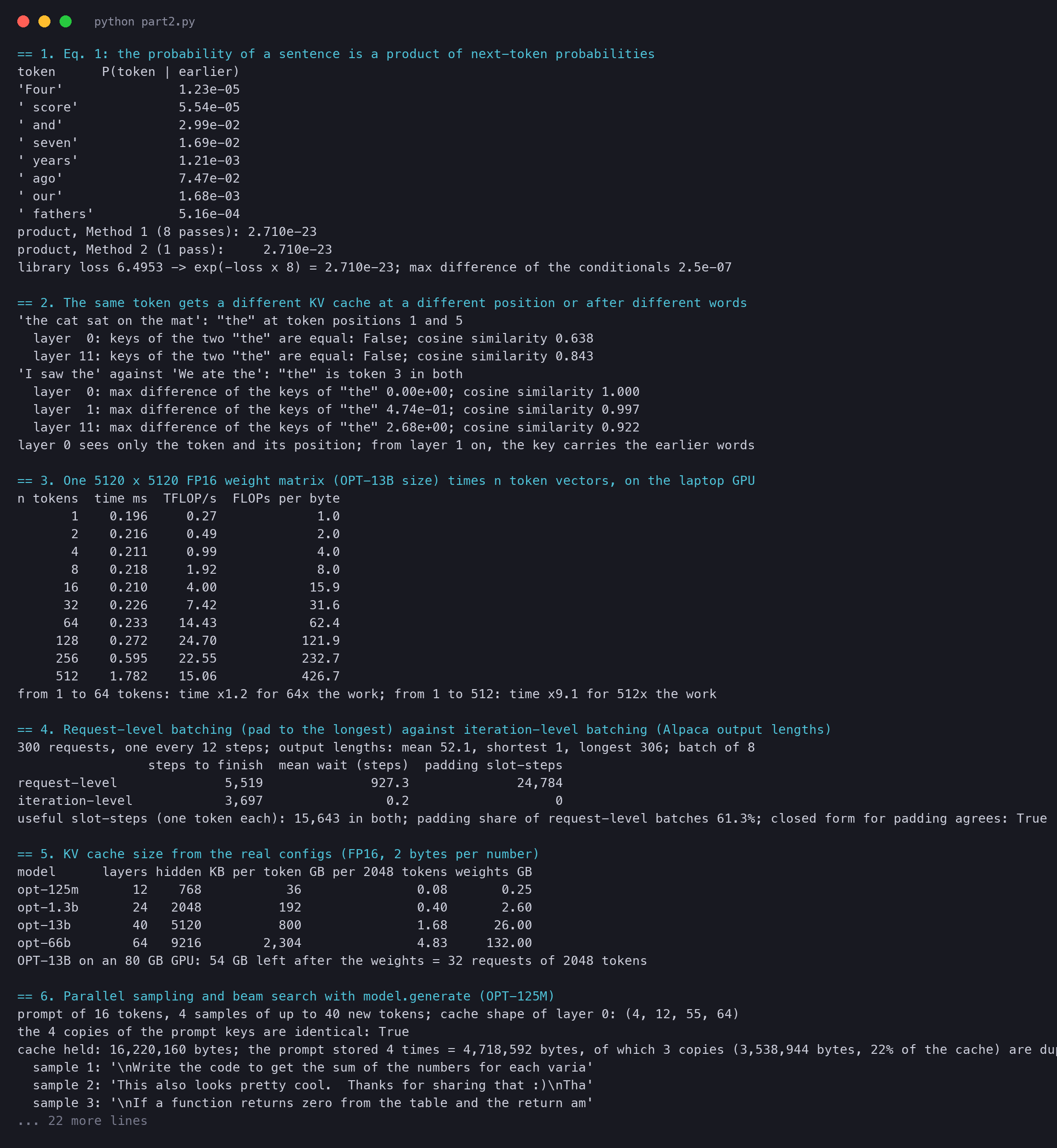
The full output of vllm_part2.py, as it ran for this article.