ViT, explained · Part 3 of 4 · Covers §3.2, §4 (opening), §4.1, Tables 1, 3 and 4, Appendix B.1 and B.1.1

Fine-tuning, Higher Resolution and the Setup

How a pre-trained ViT is adapted to a new task, why it is fine-tuned on bigger pictures, and the full training recipe behind every result. We swap the head, stretch the position embeddings, fine-tune on ten classes and solve the few-shot metric by hand.

An Image is Worth 16x16 Words: Transformers for Image Recognition at Scale. Alexey Dosovitskiy, Lucas Beyer, Alexander Kolesnikov, Dirk Weissenborn, Xiaohua Zhai, Thomas Unterthiner, Mostafa Dehghani, Matthias Minderer, Georg Heigold, Sylvain Gelly, Jakob Uszkoreit, Neil Houlsby. ICLR 2021, 2020. arXiv:2010.11929

Part 2 built ViT from pixels to a class label. A model is only half of a paper, though. The other half is how it is trained, adapted and measured, and that half decides every number in the results.

Fine-tuning: a new head for a new task#

The released ViT-B/16 checkpoint pre-trained on ImageNet-21k shows the old head. It ends in a "pre-logits" layer, a $768 \times 768$ matrix with a tanh (Part 2 met it as the library's "pooler"). The 21,843-class layer on top of it was not released. Appendix B.1.1 says what is removed:

vit_part3_finetune.py loads the ImageNet-21k checkpoint into a 10-class classifier, sets the new head to zero and runs one batch of 32 Imagenette pictures through it. (Imagenette is a small public set of 10 ImageNet classes, described in the fine-tuning run below.)

model = ViTForImageClassification.from_pretrained('google/vit-base-patch16-224-in21k', num_labels=10)
torch.nn.init.zeros_(model.classifier.weight); torch.nn.init.zeros_(model.classifier.bias)
loss = F.cross_entropy(model(pixel_values=x).logits, y); loss.backward()

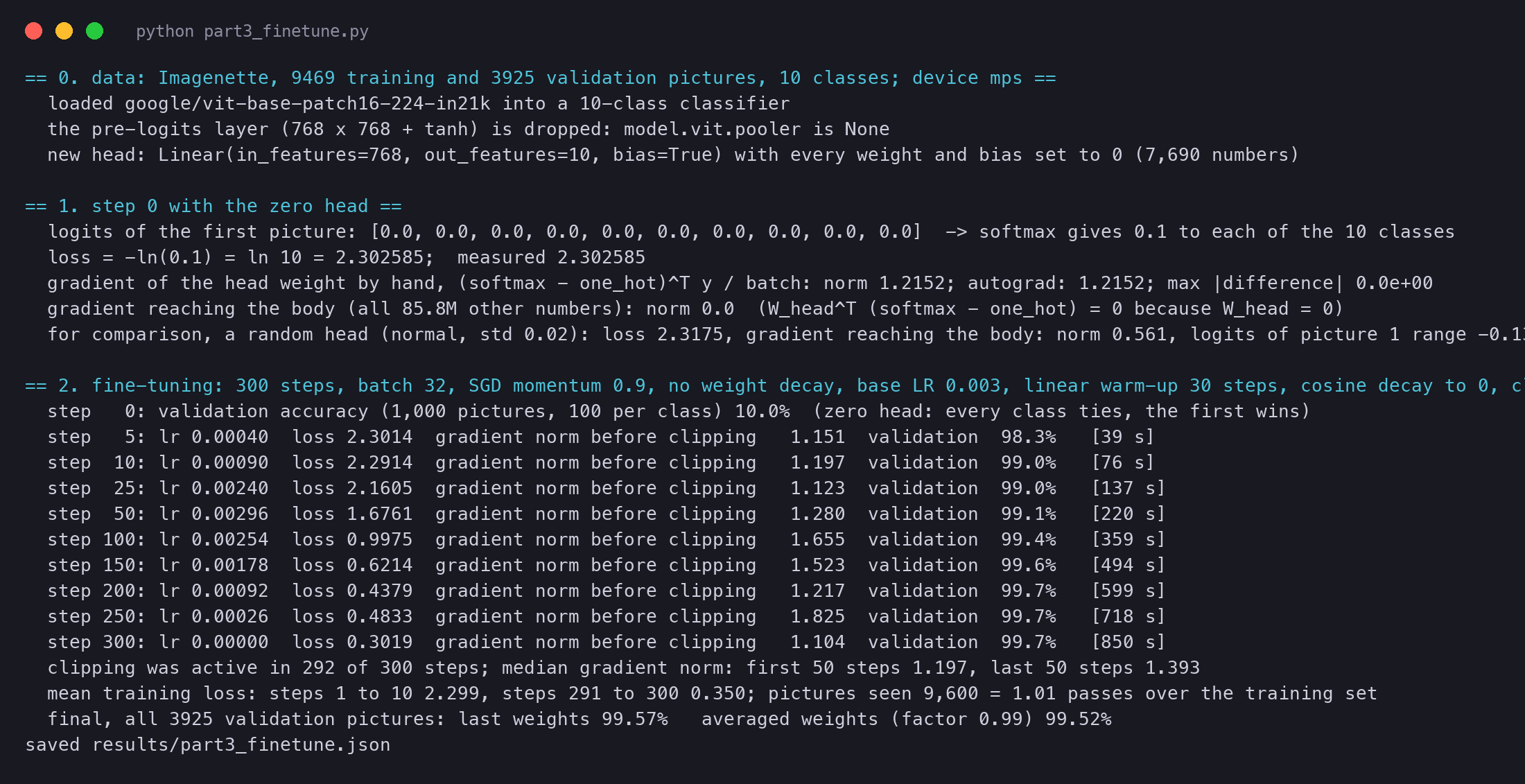
== 0. data: Imagenette, 9469 training and 3925 validation pictures, 10 classes; device mps ==
  loaded google/vit-base-patch16-224-in21k into a 10-class classifier
  the pre-logits layer (768 x 768 + tanh) is dropped: model.vit.pooler is None
  new head: Linear(in_features=768, out_features=10, bias=True) with every weight and bias set to 0 (7,690 numbers)

== 1. step 0 with the zero head ==
  logits of the first picture: [0.0, 0.0, 0.0, 0.0, 0.0, 0.0, 0.0, 0.0, 0.0, 0.0]  -> softmax gives 0.1 to each of the 10 classes
  loss = -ln(0.1) = ln 10 = 2.302585;  measured 2.302585
  gradient of the head weight by hand, (softmax - one_hot)^T y / batch: norm 1.2152; autograd: 1.2152; max |difference| 0.0e+00
  gradient reaching the body (all 85.8M other numbers): norm 0.0  (W_head^T (softmax - one_hot) = 0 because W_head = 0)
  for comparison, a random head (normal, std 0.02): loss 2.3175, gradient reaching the body: norm 0.561, logits of picture 1 range -0.13 to 0.13

The loss of the first step is exactly $\ln 10$, because ten equal scores give each class a probability of 0.1. The more surprising line is the last one: the body gets a gradient of exactly 0. The chain rule explains it. The gradient that flows back into the [class] token is the head's weight matrix times the error of each class:

Here $\mathbf{y}$ is the image representation (768 numbers) and $W_{\text{head}}$ the new $10 \times 768$ head. $\mathbf{p}$ holds the 10 predicted probabilities, and $\mathbf{t}$ is the one-hot target (1 for the right class, 0 for the rest). The head itself does get a gradient, $(\mathbf{p} - \mathbf{t})\,\mathbf{y}^\top$ averaged over the batch, because $\mathbf{y}$ is not zero. So step 1 changes only the head. From step 2 on, the head is no longer zero and the body starts to move.

A random head does the opposite. Its scores are noise (−0.13 to 0.13 here), and its loss starts above $\ln 10$, at 2.3175. That noise sends a gradient of size 0.561 into all 85.8 million pre-trained numbers on the very first step. The zero head lets the pre-trained body wait until the head has learned something sensible.

Fine-tuning at a higher resolution#

The arithmetic, with the symbols of Part 2 ($N = HW/P^2$):

So the sequence grows from 197 to 577 tokens, about 2.9 times longer. Attention compares every pair of tokens, so its pairs grow from 38,809 to 332,929, about 8.6 times. The whole forward pass of ViT-B/16 grows from about 34.9 to 110.3 billion operations. That is our estimate from the shapes, printed in the Model variants section below.

The paper cites two sources for "often beneficial". One is BiT, the ResNet baseline we meet below. The other is a paper about exactly this effect:

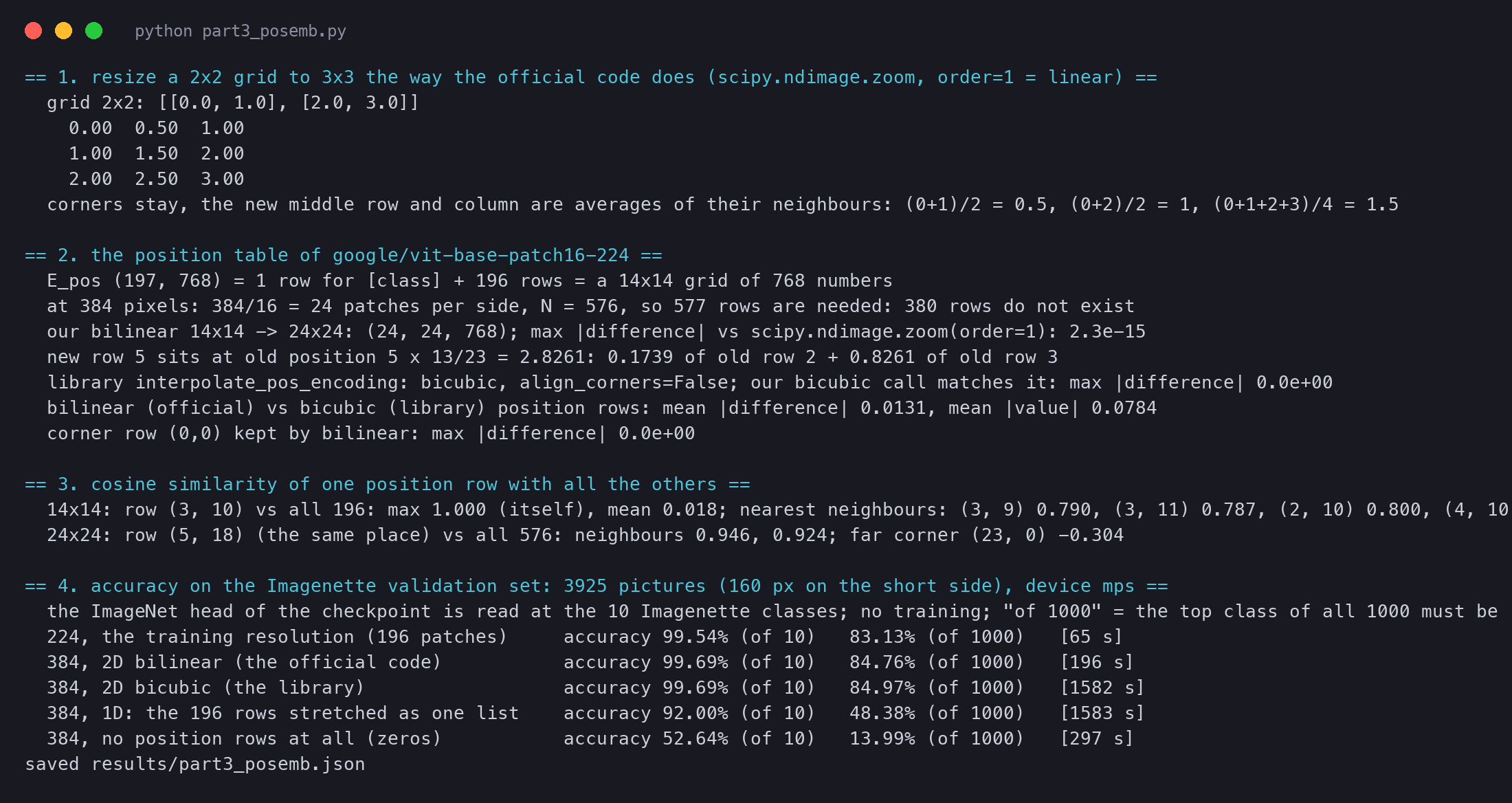
A tiny example first. The official code resizes the grid with scipy.ndimage.zoom(..., order=1), which is linear interpolation in each direction with the corner values kept. On a 2 × 2 grid of single numbers, resized to 3 × 3 (vit_part3_posemb.py):

== 1. resize a 2x2 grid to 3x3 the way the official code does (scipy.ndimage.zoom, order=1 = linear) ==
  grid 2x2: [[0.0, 1.0], [2.0, 3.0]]
    0.00  0.50  1.00
    1.00  1.50  2.00
    2.00  2.50  3.00
  corners stay, the new middle row and column are averages of their neighbours: (0+1)/2 = 0.5, (0+2)/2 = 1, (0+1+2+3)/4 = 1.5

Check it by hand. The four corners keep their values 0, 1, 2 and 3. The new top-middle value sits halfway between 0 and 1, so it is 0.5. The centre sits halfway between all four, so it is $(0 + 1 + 2 + 3)/4 = 1.5$.

The formula. For one new grid row $i$ out of $n_{\text{new}}$, the place on the old grid of $n_{\text{old}}$ rows is

where $\lfloor y \rfloor$ is $y$ rounded down, and $\delta$ is how far the new row sits past that old row. The same rule then runs along the columns. Each "row" here is a whole vector of 768 numbers, so the mix is done number by number. For ViT-B/16 at 384, $n_{\text{old}} = 14$ and $n_{\text{new}} = 24$. New row 5 sits at $5 \times 13/23 = 2.8261$, so it takes 0.1739 of old row 2 and 0.8261 of old row 3.

The real table. We wrote this rule as a plain loop and ran it on the 14 × 14 × 768 position grid of google/vit-base-patch16-224. Then we compared it with SciPy and with the library:

== 2. the position table of google/vit-base-patch16-224 ==
  E_pos (197, 768) = 1 row for [class] + 196 rows = a 14x14 grid of 768 numbers
  at 384 pixels: 384/16 = 24 patches per side, N = 576, so 577 rows are needed: 380 rows do not exist
  our bilinear 14x14 -> 24x24: (24, 24, 768); max |difference| vs scipy.ndimage.zoom(order=1): 2.3e-15
  new row 5 sits at old position 5 x 13/23 = 2.8261: 0.1739 of old row 2 + 0.8261 of old row 3
  library interpolate_pos_encoding: bicubic, align_corners=False; our bicubic call matches it: max |difference| 0.0e+00
  bilinear (official) vs bicubic (library) position rows: mean |difference| 0.0131, mean |value| 0.0784
  corner row (0,0) kept by bilinear: max |difference| 0.0e+00

Our loop equals SciPy's resize to $2 \times 10^{-15}$, which is the rounding of 64-bit numbers. The Hugging Face library does something slightly different: it uses bicubic interpolation, not bilinear. The two tables differ by 0.0131 on average, against an average size of 0.0784 for the numbers themselves. So the official and the library versions are close but not the same.

To see what the stretch keeps, take one position row and compare it, by cosine similarity, with every other row. In the 14 × 14 grid, row (3, 10) is most like its four neighbours (0.79 to 0.81) and unlike the far corner (−0.29). After the stretch, the same place on the 24 × 24 grid shows the same pattern, only smoother. Its neighbours are now closer (0.92 to 0.95), because they are made from the same old rows.

Does it work? We ran the ImageNet-fine-tuned ViT-B/16 on the 3,925 validation pictures of Imagenette. We used 224 and 384 pixels, and five versions of the position table. There is no training here at all; only the position table changes.

== 4. accuracy on the Imagenette validation set: 3925 pictures (160 px on the short side), device mps ==
  the ImageNet head of the checkpoint is read at the 10 Imagenette classes; no training; "of 1000" = the top class of all 1000 must be right
  224, the training resolution (196 patches)     accuracy 99.54% (of 10)   83.13% (of 1000)   [65 s]
  384, 2D bilinear (the official code)           accuracy 99.69% (of 10)   84.76% (of 1000)   [196 s]
  384, 2D bicubic (the library)                  accuracy 99.69% (of 10)   84.97% (of 1000)   [1582 s]
  384, 1D: the 196 rows stretched as one list    accuracy 92.00% (of 10)   48.38% (of 1000)   [1583 s]
  384, no position rows at all (zeros)           accuracy 52.64% (of 10)   13.99% (of 1000)   [297 s]

The two 2D stretches keep the model working at 384. Over all 1,000 ImageNet classes, accuracy is 84.76% with the official bilinear table and 84.97% with the library's bicubic one, against 83.13% at 224. Read at only the 10 Imagenette classes, all three are almost perfect (99.54% to 99.69%).

The wrong stretch is a disaster. Stretching the 196 rows as one list of 576 drops the accuracy to 48.38%. A 1D stretch treats the last patch of one grid row and the first patch of the next as neighbours. So most new rows land in the wrong place. With no position rows at all the model falls to 13.99%; Part 2 showed why, since attention alone sees only a bag of patches.

Two honest limits. This model was never fine-tuned at 384, and the paper always fine-tunes after the stretch. Our numbers show only that the stretched table is a good start. And Imagenette stores its pictures at 160 pixels, so at 384 they are only upscaled, with no new detail. The small gain at 384 cannot come from detail. It fits the explanation of Touvron et al. that objects simply look bigger.

The times in brackets include waiting for another job on the same GPU, so they say nothing about speed.

The experiments: three model families#

Datasets#

Model variants and the "/16" in the name#

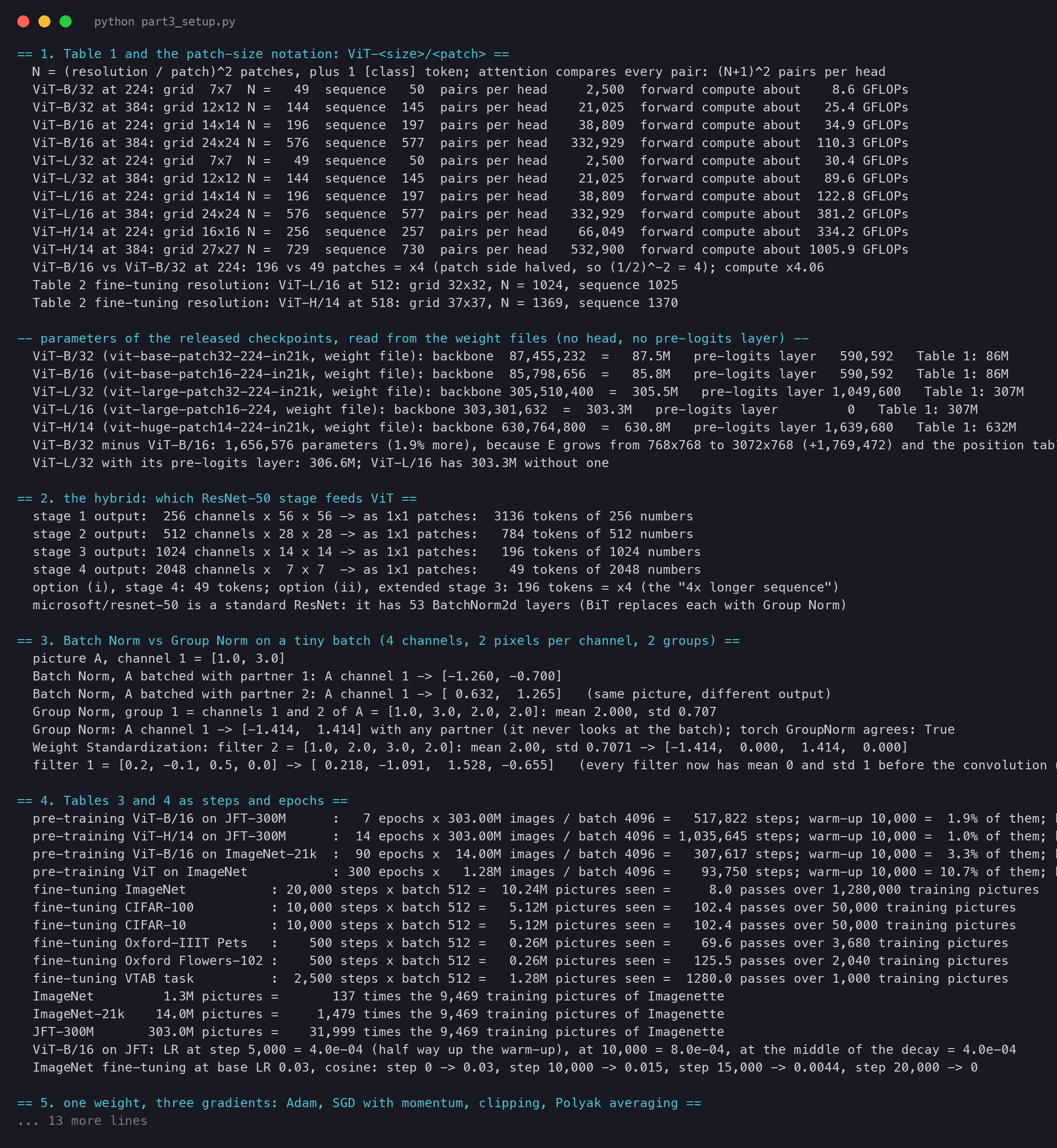
Part 2 counted the parameters of each size from a formula. Here we add the patch size and the resolution. vit_part3_setup.py computes the sequence length and an estimate of the forward compute from the shapes, and counts the numbers in each released weight file:

== 1. Table 1 and the patch-size notation: ViT-<size>/<patch> ==
  N = (resolution / patch)^2 patches, plus 1 [class] token; attention compares every pair: (N+1)^2 pairs per head
  ViT-B/32 at 224: grid  7x7  N =   49  sequence   50  pairs per head     2,500  forward compute about    8.6 GFLOPs
  ViT-B/32 at 384: grid 12x12 N =  144  sequence  145  pairs per head    21,025  forward compute about   25.4 GFLOPs
  ViT-B/16 at 224: grid 14x14 N =  196  sequence  197  pairs per head    38,809  forward compute about   34.9 GFLOPs
  ViT-B/16 at 384: grid 24x24 N =  576  sequence  577  pairs per head   332,929  forward compute about  110.3 GFLOPs
  ViT-L/32 at 224: grid  7x7  N =   49  sequence   50  pairs per head     2,500  forward compute about   30.4 GFLOPs
  ViT-L/32 at 384: grid 12x12 N =  144  sequence  145  pairs per head    21,025  forward compute about   89.6 GFLOPs
  ViT-L/16 at 224: grid 14x14 N =  196  sequence  197  pairs per head    38,809  forward compute about  122.8 GFLOPs
  ViT-L/16 at 384: grid 24x24 N =  576  sequence  577  pairs per head   332,929  forward compute about  381.2 GFLOPs
  ViT-H/14 at 224: grid 16x16 N =  256  sequence  257  pairs per head    66,049  forward compute about  334.2 GFLOPs
  ViT-H/14 at 384: grid 27x27 N =  729  sequence  730  pairs per head   532,900  forward compute about 1005.9 GFLOPs
  ViT-B/16 vs ViT-B/32 at 224: 196 vs 49 patches = x4 (patch side halved, so (1/2)^-2 = 4); compute x4.06
  Table 2 fine-tuning resolution: ViT-L/16 at 512: grid 32x32, N = 1024, sequence 1025
  Table 2 fine-tuning resolution: ViT-H/14 at 518: grid 37x37, N = 1369, sequence 1370

-- parameters of the released checkpoints, read from the weight files (no head, no pre-logits layer) --
  ViT-B/32 (vit-base-patch32-224-in21k, weight file): backbone  87,455,232  =   87.5M   pre-logits layer   590,592   Table 1: 86M
  ViT-B/16 (vit-base-patch16-224-in21k, weight file): backbone  85,798,656  =   85.8M   pre-logits layer   590,592   Table 1: 86M
  ViT-L/32 (vit-large-patch32-224-in21k, weight file): backbone 305,510,400  =  305.5M   pre-logits layer 1,049,600   Table 1: 307M
  ViT-L/16 (vit-large-patch16-224, weight file): backbone 303,301,632  =  303.3M   pre-logits layer         0   Table 1: 307M
  ViT-H/14 (vit-huge-patch14-224-in21k, weight file): backbone 630,764,800  =  630.8M   pre-logits layer 1,639,680   Table 1: 632M
  ViT-B/32 minus ViT-B/16: 1,656,576 parameters (1.9% more), because E grows from 768x768 to 3072x768 (+1,769,472) and the position table shrinks from 197 to 50 rows (-112,896)
  ViT-L/32 with its pre-logits layer: 306.6M; ViT-L/16 has 303.3M without one

Three things stand out. First, ViT-B/16 needs 4.06 times the compute of ViT-B/32 at 224 pixels, almost exactly the factor 4 of the paper's sentence. The extra 0.06 comes from attention, whose cost grows with the square of the sequence.

Second, ViT-B/32 has 1.9% more parameters than ViT-B/16, not fewer: its patch embedding is $3{,}072 \times 768$ instead of $768 \times 768$. Parameters and compute are separate dials.

Third, the 307M of ViT-Large in Table 1 is close to ViT-L/32 with its pre-logits layer (306.6M). ViT-L/16 has 303.3M without one; its only cached file is the ImageNet fine-tuned one, which has no pre-logits layer. Part 2 already flagged this gap. The table may count a different version; we cannot tell which.

The CNN baselines: ResNet (BiT) and Noisy Student#

The difference fits on a few numbers. Picture A has 4 channels of 2 pixels each. We normalise it once together with one partner picture and once with another:

== 3. Batch Norm vs Group Norm on a tiny batch (4 channels, 2 pixels per channel, 2 groups) ==
  picture A, channel 1 = [1.0, 3.0]
  Batch Norm, A batched with partner 1: A channel 1 -> [-1.260, -0.700]
  Batch Norm, A batched with partner 2: A channel 1 -> [ 0.632,  1.265]   (same picture, different output)
  Group Norm, group 1 = channels 1 and 2 of A = [1.0, 3.0, 2.0, 2.0]: mean 2.000, std 0.707
  Group Norm: A channel 1 -> [-1.414,  1.414] with any partner (it never looks at the batch); torch GroupNorm agrees: True
  Weight Standardization: filter 2 = [1.0, 2.0, 3.0, 2.0]: mean 2.00, std 0.7071 -> [-1.414,  0.000,  1.414,  0.000]
  filter 1 = [0.2, -0.1, 0.5, 0.0] -> [ 0.218, -1.091,  1.528, -0.655]   (every filter now has mean 0 and std 1 before the convolution uses it)

With Batch Norm, the same picture A gives $[-1.260, -0.700]$ in one batch and $[0.632, 1.265]$ in another. Its output depends on a stranger. With Group Norm, channels 1 and 2 of A form a group with values $1, 3, 2, 2$: mean 2, spread $\sqrt{(1 + 1 + 0 + 0)/4} = 0.707$. So channel 1 becomes $(1 - 2)/0.707 = -1.414$ and $(3 - 2)/0.707 = 1.414$, whatever the batch. The released microsoft/resnet-50 that Part 1 ran is a standard ResNet with 53 Batch Norm layers; ResNet (BiT) swaps each of them for Group Norm.

The BiT paper gives the reason in its own words:

The second opponent appears in Section 4.2 (Part 4): Noisy Student, which the paper calls the state of the art on ImageNet at the time. It is a different kind of CNN trained in a different way:

The hybrids: which ResNet stage feeds ViT#

The real ResNet-50 shows the four grids on one Imagenette picture:

== 2. the hybrid: which ResNet-50 stage feeds ViT ==
  stage 1 output:  256 channels x 56 x 56 -> as 1x1 patches:  3136 tokens of 256 numbers
  stage 2 output:  512 channels x 28 x 28 -> as 1x1 patches:   784 tokens of 512 numbers
  stage 3 output: 1024 channels x 14 x 14 -> as 1x1 patches:   196 tokens of 1024 numbers
  stage 4 output: 2048 channels x  7 x 7  -> as 1x1 patches:    49 tokens of 2048 numbers
  option (i), stage 4: 49 tokens; option (ii), extended stage 3: 196 tokens = x4 (the "4x longer sequence")
  microsoft/resnet-50 is a standard ResNet: it has 53 BatchNorm2d layers (BiT replaces each with Group Norm)

Pre-training: Adam, a big batch and strong weight decay#

Adam, by hand. The intuition: a hiker in fog keeps a running sense of which way is downhill ($m$), and of how bumpy the ground has been ($v$). Steps are long on smooth ground and short on bumpy ground. For one weight $w$ with gradient $g_t$ at step $t$:

Here $m_t$ is the running average of the gradient with memory $\beta_1 = 0.9$, and $v_t$ the running average of the squared gradient with memory $\beta_2 = 0.999$. $\hat m_t$ and $\hat v_t$ are the same averages, corrected for starting at 0. $\eta$ is the learning rate, and $\epsilon$ a tiny number ($10^{-8}$) that avoids a division by zero. With three gradients $0.5, -0.1, 0.3$ and $\eta = 0.001$:

  Adam t=1: g= 0.50  m=0.0500  v=0.000250  m_hat=0.5000  v_hat=0.2500  step = lr*m_hat/sqrt(v_hat) = 0.001000  w=0.999000
  Adam t=2: g=-0.10  m=0.0350  v=0.000260  m_hat=0.1842  v_hat=0.1299  step = lr*m_hat/sqrt(v_hat) = 0.000511  w=0.998489
  Adam t=3: g= 0.30  m=0.0615  v=0.000349  m_hat=0.2269  v_hat=0.1166  step = lr*m_hat/sqrt(v_hat) = 0.000665  w=0.997824
  torch.optim.Adam after the same three gradients: w=0.997824  (ours 0.997824)

Check step 1 with a pencil: $m_1 = 0.1 \times 0.5 = 0.05$ and $v_1 = 0.001 \times 0.25 = 0.00025$. The corrections divide by $1 - 0.9 = 0.1$ and $1 - 0.999 = 0.001$, giving $\hat m_1 = 0.5$ and $\hat v_1 = 0.25$. The step is $0.001 \times 0.5 / \sqrt{0.25} = 0.001$. The first step of Adam is always exactly $\eta$ long, whatever the size of the gradient. That is why a warm-up matters: without it, every weight jumps by the full learning rate at once.

Turned into steps, the table reads like this (vit_part3_setup.py; the ImageNet training set is 1.28 million pictures):

  pre-training ViT-B/16 on JFT-300M      :   7 epochs x 303.00M images / batch 4096 =   517,822 steps; warm-up 10,000 =  1.9% of them; base LR 0.0008, linear decay
  pre-training ViT-H/14 on JFT-300M      :  14 epochs x 303.00M images / batch 4096 = 1,035,645 steps; warm-up 10,000 =  1.0% of them; base LR 0.0003, linear decay
  pre-training ViT-B/16 on ImageNet-21k  :  90 epochs x  14.00M images / batch 4096 =   307,617 steps; warm-up 10,000 =  3.3% of them; base LR 0.001, linear decay
  pre-training ViT on ImageNet           : 300 epochs x   1.28M images / batch 4096 =    93,750 steps; warm-up 10,000 = 10.7% of them; base LR 0.003, cosine decay
  ViT-B/16 on JFT: LR at step 5,000 = 4.0e-04 (half way up the warm-up), at 10,000 = 8.0e-04, at the middle of the decay = 4.0e-04

The 10,000 warm-up steps are under 2% of a JFT run, but almost 11% of an ImageNet run. One rule fits very different runs. The learning rate itself is a ramp up and a long line down:

Fine-tuning: SGD with momentum, cosine decay, clipping#

SGD with momentum and Polyak averaging, by hand. For one weight with velocity $u$, momentum $\mu = 0.9$ and learning rate $\eta$:

where $u_t$ is the velocity, a running sum of gradients that forgets 10% per step, and $\bar w_t$ is the Polyak average with factor $\beta$. The same three gradients as before, with $\eta = 0.01$, and an average with $\beta = 0.9$ of five weight values:

  SGD momentum 0.9, lr 0.01, t=1: g= 0.50  velocity = 0.9*velocity + g = 0.5000  w = w - lr*velocity = 0.99500
  SGD momentum 0.9, lr 0.01, t=2: g=-0.10  velocity = 0.9*velocity + g = 0.3500  w = w - lr*velocity = 0.99150
  SGD momentum 0.9, lr 0.01, t=3: g= 0.30  velocity = 0.9*velocity + g = 0.6150  w = w - lr*velocity = 0.98535
  torch.optim.SGD(momentum=0.9) after the same gradients: w=0.98535  (ours 0.98535)
  Polyak (exponential) averaging, factor 0.9: weights [1.0, 1.2, 0.9, 1.1, 1.05] -> averages [1.0, 1.02, 1.008, 1.0172, 1.0205]
  a factor of 0.9999 averages over roughly the last 1/(1 - 0.9999) = 10,000 steps

At step 2 the gradient is $-0.1$, uphill, but the velocity is still $0.9 \times 0.5 - 0.1 = 0.35$, so the weight keeps moving down. That is momentum: one contrary batch does not reverse the direction. The Polyak average of the jittering weights $1.00, 1.20, 0.90, 1.10, 1.05$ moves only from 1.0 to 1.0205. A factor of 0.9999 averages over roughly the last 10,000 steps, half of an ImageNet fine-tuning run of 20,000 steps.

Cosine decay and clipping, in numbers. With base learning rate $\eta_0$ and $T$ steps, cosine decay sets step $t$ to

which is $\eta_0$ at $t = 0$, $\eta_0/2$ halfway, and 0 at the end. For ImageNet with $\eta_0 = 0.03$ and $T = 20{,}000$: 0.03, then 0.015 at step 10,000, 0.0044 at step 15,000, and 0 at step 20,000. Clipping uses the global norm $\lVert g \rVert = \sqrt{\sum_i g_i^2}$ over all weights, and multiplies the gradient by $\min(1, 1/\lVert g \rVert)$. With two tensors of gradients $[3, 0]$ and $[4]$:

  clipping at global norm 1: gradients of two tensors [3, 0] and [4]; global norm sqrt(9 + 0 + 16) = 5.0 > 1, so every gradient is multiplied by 1/5: [0.6, 0.0] and [0.8]; direction kept, length 1
  torch.nn.utils.clip_grad_norm_: [0.6, 0.0] and [0.8]

The length is $\sqrt{9 + 0 + 16} = 5$, so every number is divided by 5: $[0.6, 0]$ and $[0.8]$, a vector of length 1 that points the same way. Table 4 in steps and passes over the data:

  fine-tuning ImageNet           : 20,000 steps x batch 512 =  10.24M pictures seen =     8.0 passes over 1,280,000 training pictures
  fine-tuning CIFAR-100          : 10,000 steps x batch 512 =   5.12M pictures seen =   102.4 passes over 50,000 training pictures
  fine-tuning CIFAR-10           : 10,000 steps x batch 512 =   5.12M pictures seen =   102.4 passes over 50,000 training pictures
  fine-tuning Oxford-IIIT Pets   :    500 steps x batch 512 =   0.26M pictures seen =    69.6 passes over 3,680 training pictures
  fine-tuning Oxford Flowers-102 :    500 steps x batch 512 =   0.26M pictures seen =   125.5 passes over 2,040 training pictures
  fine-tuning VTAB task          :  2,500 steps x batch 512 =   1.28M pictures seen =  1280.0 passes over 1,000 training pictures
  ImageNet fine-tuning at base LR 0.03, cosine: step 0 -> 0.03, step 10,000 -> 0.015, step 15,000 -> 0.0044, step 20,000 -> 0

These counts use the standard training-set sizes of each benchmark. Pets is seen about 70 times, and each 1,000-example VTAB task 1,280 times. Small tasks get many passes but few steps.

Our fine-tuning run#

The paper's fine-tuning runs are far beyond one computer: 20,000 steps of 512 pictures at 384 pixels. We kept the pieces of the recipe and shrank the scale. We start from the ImageNet-21k checkpoint of ViT-B/16 with the zero head shown above. We fine-tune it on Imagenette, a public set of 10 easy ImageNet classes. They are tench, English springer, cassette player, chain saw, church, French horn, garbage truck, gas pump, golf ball and parachute. It has 9,469 training and 3,925 validation pictures, stored at 160 pixels on the short side.

vit_part3_finetune.py runs 300 steps of 32 pictures at 224 pixels, so the model sees 9,600 pictures, about one pass over the training set. The pieces follow Table 4: SGD with momentum 0.9, no weight decay, cosine decay and clipping at global norm 1. We also keep a running average of the weights.

Three choices are ours. The batch is 32 instead of 512. There is a short linear warm-up of 30 steps, which Table 4 does not list. And the learning rate is 0.003, a value from Table 4's grid, picked without a search.

opt = torch.optim.SGD(model.parameters(), lr=LR, momentum=0.9, weight_decay=0.0)
for step in range(1, STEPS + 1):
    for g in opt.param_groups:
        g['lr'] = lr_at(step - 1)                               # warm-up, then cosine to 0
    loss = F.cross_entropy(model(pixel_values=x).logits, y)
    opt.zero_grad(); loss.backward()
    torch.nn.utils.clip_grad_norm_(model.parameters(), 1.0)    # global norm 1
    opt.step()
    for pe, pm in zip(ema.parameters(), model.parameters()):   # Polyak average, factor 0.99
        pe.mul_(0.99).add_(pm.detach(), alpha=0.01)

== 2. fine-tuning: 300 steps, batch 32, SGD momentum 0.9, no weight decay, base LR 0.003, linear warm-up 30 steps, cosine decay to 0, clip at global norm 1.0, weight average factor 0.99, random horizontal flips ==
  step   0: validation accuracy (1,000 pictures, 100 per class) 10.0%  (zero head: every class ties, the first wins)
  step   5: lr 0.00040  loss 2.3014  gradient norm before clipping   1.151  validation  98.3%   [39 s]
  step  10: lr 0.00090  loss 2.2914  gradient norm before clipping   1.197  validation  99.0%   [76 s]
  step  25: lr 0.00240  loss 2.1605  gradient norm before clipping   1.123  validation  99.0%   [137 s]
  step  50: lr 0.00296  loss 1.6761  gradient norm before clipping   1.280  validation  99.1%   [220 s]
  step 100: lr 0.00254  loss 0.9975  gradient norm before clipping   1.655  validation  99.4%   [359 s]
  step 150: lr 0.00178  loss 0.6214  gradient norm before clipping   1.523  validation  99.6%   [494 s]
  step 200: lr 0.00092  loss 0.4379  gradient norm before clipping   1.217  validation  99.7%   [599 s]
  step 250: lr 0.00026  loss 0.4833  gradient norm before clipping   1.825  validation  99.7%   [718 s]
  step 300: lr 0.00000  loss 0.3019  gradient norm before clipping   1.104  validation  99.7%   [850 s]
  clipping was active in 292 of 300 steps; median gradient norm: first 50 steps 1.197, last 50 steps 1.393
  mean training loss: steps 1 to 10 2.299, steps 291 to 300 0.350; pictures seen 9,600 = 1.01 passes over the training set

Read the loss and the accuracy side by side. After only 5 steps, validation accuracy jumps from 10.0% to 98.3%, while the loss has barely moved from $\ln 10$ (2.3014). Accuracy only asks whether the right class has the highest score. The loss asks how sure the model is. After 5 small steps the head already points the right way, but its scores are still small, since the loss is still close to $\ln 10$. The other 295 steps mostly make the model confident: the mean loss of the last 10 steps is 0.350.

Two numbers deserve a comment. Clipping was active in 292 of the 300 steps. The median gradient norm was 1.197 over the first 50 steps and 1.393 over the last 50, above the cap of 1. At our batch of 32, the cap of 1 works more like a fixed step length than like a rare guard. A batch of 512 averages more pictures, so its gradient is less noisy and may hit the cap less often; we did not measure that.

The weight average with factor 0.99 ended at 99.52%, against 99.57% for the last weights. On a task this easy, the average has no jitter to remove.

What this run cannot show: Imagenette is tiny and easy. Its ten classes are among the labels of ImageNet-21k, so the body has seen them before. We used one run, one learning rate and 224 pixels instead of 384. The paper's fine-tuning numbers come from much harder tasks, many runs and a learning-rate search. Our run shows the mechanics of the recipe, not its value.

Metrics: fine-tuning accuracy and few-shot accuracy#

The closed form. The intuition: draw the best straight line through the training points. "Best" means the smallest total squared miss, plus a small fine for steep lines. For the few-shot layer:

where:

• $X$ has one row per training picture: its frozen representation of $d$ numbers, plus a 1 at the end for a bias. So it is $n \times (d + 1)$;
• $Y$ is $n \times K$: row $i$ holds +1 in the column of picture $i$'s class and −1 in the other $K - 1$ columns;
• $W$ is the linear layer, $(d + 1) \times K$; $XW$ are the predicted scores;
• $\lambda \geq 0$ sets the fine for large weights, and $I$ is the identity matrix;
• $\lVert \cdot \rVert^2$ is the sum of squares of all entries.

A new picture with representation $x$ gets the $K$ scores $xW$, and the largest score names its class. The formula comes from one line of calculus: set the gradient $2X^\top(XW - Y) + 2\lambda W$ to zero, and you get $(X^\top X + \lambda I)\,W = X^\top Y$. Solving that linear system is all the "training" there is.

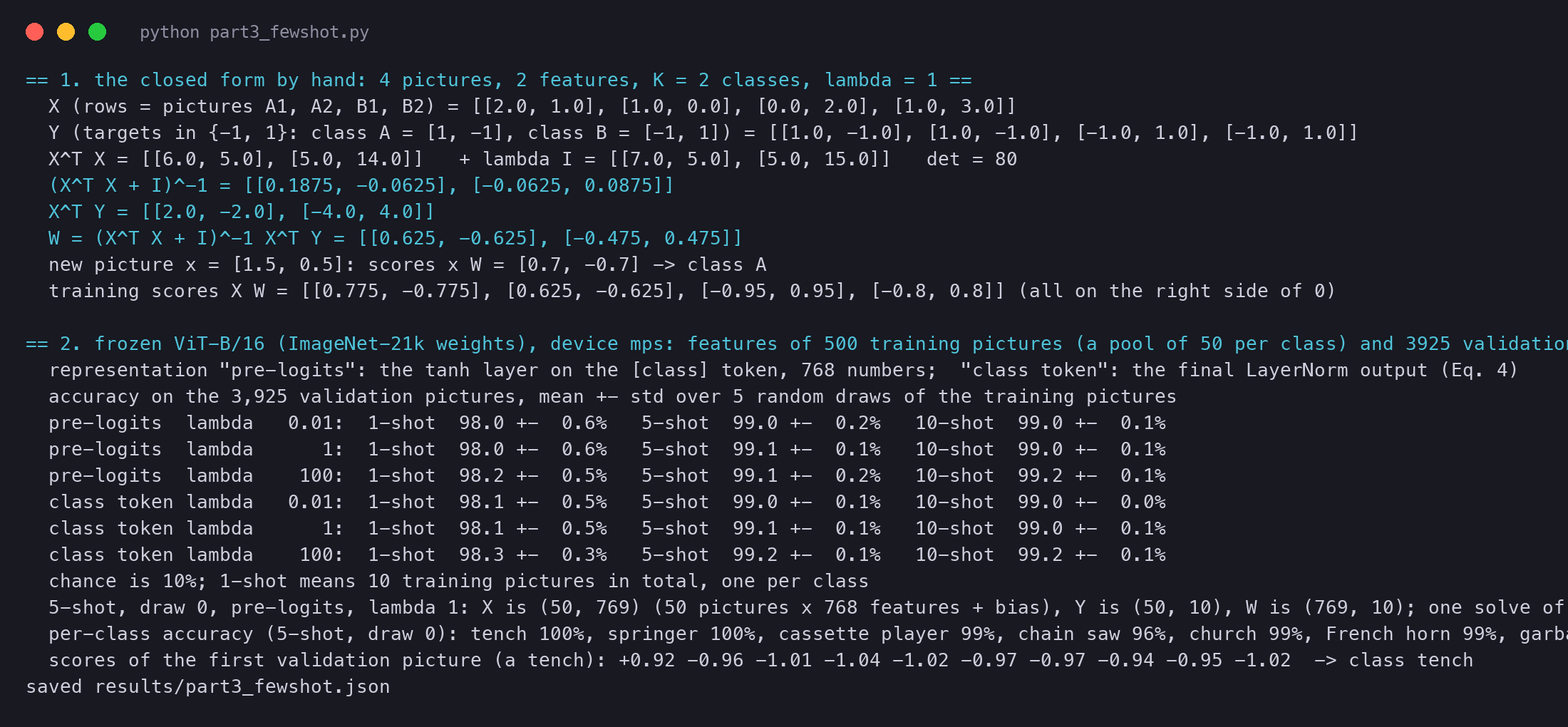
A tiny example by hand (vit_part3_fewshot.py). Four pictures have two features each, two of class A and two of class B. We use $\lambda = 1$ and no bias column, to keep the sums short.

== 1. the closed form by hand: 4 pictures, 2 features, K = 2 classes, lambda = 1 ==
  X (rows = pictures A1, A2, B1, B2) = [[2.0, 1.0], [1.0, 0.0], [0.0, 2.0], [1.0, 3.0]]
  Y (targets in {-1, 1}: class A = [1, -1], class B = [-1, 1]) = [[1.0, -1.0], [1.0, -1.0], [-1.0, 1.0], [-1.0, 1.0]]
  X^T X = [[6.0, 5.0], [5.0, 14.0]]   + lambda I = [[7.0, 5.0], [5.0, 15.0]]   det = 80
  (X^T X + I)^-1 = [[0.1875, -0.0625], [-0.0625, 0.0875]]
  X^T Y = [[2.0, -2.0], [-4.0, 4.0]]
  W = (X^T X + I)^-1 X^T Y = [[0.625, -0.625], [-0.475, 0.475]]
  new picture x = [1.5, 0.5]: scores x W = [0.7, -0.7] -> class A
  training scores X W = [[0.775, -0.775], [0.625, -0.625], [-0.95, 0.95], [-0.8, 0.8]] (all on the right side of 0)

Check it with a pencil. The top-left entry of $X^\top X$ is $2^2 + 1^2 + 0^2 + 1^2 = 6$, and the off-diagonal entry is $2 \cdot 1 + 1 \cdot 0 + 0 \cdot 2 + 1 \cdot 3 = 5$. Adding $\lambda = 1$ on the diagonal gives $\begin{bmatrix} 7 & 5 \\ 5 & 15 \end{bmatrix}$, with determinant $7 \cdot 15 - 5 \cdot 5 = 80$, so its inverse is $\tfrac{1}{80}\begin{bmatrix} 15 & -5 \\ -5 & 7 \end{bmatrix}$. The first column of $X^\top Y$ is $(2 + 1 - 0 - 1,\ 1 + 0 - 2 - 3) = (2, -4)$. So the first column of $W$ is

The new picture $(1.5, 0.5)$ scores $1.5 \times 0.625 + 0.5 \times (-0.475) = 0.7$ for class A and $-0.7$ for class B, so it is class A. With two classes, the second column is just the first with its sign flipped. With $K$ classes, each column is its own "this class against all the others" line.

The real thing. We froze ViT-B/16 with its ImageNet-21k weights, never trained on Imagenette. We computed the representation of 500 training pictures (a pool of 50 per class) and of all 3,925 validation pictures. Then we drew 1, 5 or 10 pictures per class from the pool, five times each, and solved the formula above:

X = np.hstack([features[idx], np.ones((len(idx), 1))])     # n x 769: 768 features and a bias
Y = -np.ones((len(idx), 10)); Y[np.arange(len(idx)), labels[idx]] = 1
W = np.linalg.solve(X.T @ X + lam * np.eye(769), X.T @ Y)  # the closed form
pred = (np.hstack([val_features, ones]) @ W).argmax(1)

== 2. frozen ViT-B/16 (ImageNet-21k weights), device mps: features of 500 training pictures (a pool of 50 per class) and 3925 validation pictures ==
  representation "pre-logits": the tanh layer on the [class] token, 768 numbers;  "class token": the final LayerNorm output (Eq. 4)
  accuracy on the 3,925 validation pictures, mean +- std over 5 random draws of the training pictures
  pre-logits  lambda   0.01:  1-shot  98.0 +-  0.6%   5-shot  99.0 +-  0.2%   10-shot  99.0 +-  0.1%
  pre-logits  lambda      1:  1-shot  98.0 +-  0.6%   5-shot  99.1 +-  0.1%   10-shot  99.0 +-  0.1%
  pre-logits  lambda    100:  1-shot  98.2 +-  0.5%   5-shot  99.1 +-  0.2%   10-shot  99.2 +-  0.1%
  class token lambda   0.01:  1-shot  98.1 +-  0.5%   5-shot  99.0 +-  0.1%   10-shot  99.0 +-  0.0%
  class token lambda      1:  1-shot  98.1 +-  0.5%   5-shot  99.1 +-  0.1%   10-shot  99.0 +-  0.1%
  class token lambda    100:  1-shot  98.3 +-  0.3%   5-shot  99.2 +-  0.1%   10-shot  99.2 +-  0.1%
  chance is 10%; 1-shot means 10 training pictures in total, one per class
  5-shot, draw 0, pre-logits, lambda 1: X is (50, 769) (50 pictures x 768 features + bias), Y is (50, 10), W is (769, 10); one solve of a 769x769 system
  per-class accuracy (5-shot, draw 0): tench 100%, springer 100%, cassette player 99%, chain saw 96%, church 99%, French horn 99%, garbage truck 99%, gas pump 99%, golf ball 99%, parachute 99%
  scores of the first validation picture (a tench): +0.92 -0.96 -1.01 -1.04 -1.02 -0.97 -0.97 -0.94 -0.95 -1.02  -> class tench

One picture per class, ten pictures in all, already gives 98.0% on 3,925 new pictures. Five per class gives 99.1%. The value of $\lambda$ hardly matters here (98.0% to 98.3% at 1-shot), and the two choices of representation agree within 0.2 points. The scores of one tench picture show the targets at work: +0.92 for tench and about −1 for every other class.

Do not read these numbers as "ViT learns anything from one picture". Imagenette is easy: ten very different objects, and all ten are ImageNet classes, so the ImageNet-21k pre-training already saw labelled pictures of each of them. The test shows something narrower and still useful.

A frozen representation that already separates the classes needs only a linear layer and a handful of examples. The closed form finds that layer in one solve. The paper uses the same metric on harder tasks, where models differ more. Part 4 runs it across model sizes.

Few-shot and fine-tuning measure different things. Fine-tuning asks how good the model can become on a task; few-shot asks how good its frozen vectors already are. The paper reports fine-tuning in its main tables. It uses few-shot where it must test many models, because one solve of a linear system is far cheaper than thousands of training steps.

Next, in Part 4: the results. Table 2 pits ViT-H/14 and ViT-L/16 against BiT-L and Noisy Student, and Figure 2 breaks down VTAB by group. Figures 3 and 4 answer the central question: how much data does ViT need to beat a ResNet? Continue to Part 4.

Run it yourself

Every number in this part comes from four scripts in code/papers/vit/. vit_part3_setup.py does the arithmetic of Tables 1, 3 and 4, the optimizer steps and the normalisation example. It also runs ResNet-50 once (about a minute on a CPU). vit_part3_posemb.py stretches the position table and scores five versions of it on Imagenette. vit_part3_fewshot.py solves the few-shot problem on frozen features.

vit_part3_finetune.py fine-tunes ViT-B/16 for 300 steps. The last three use the Imagenette set (imagenette2-160, from the fast.ai datasets) and a GPU if there is one.

bashCopy

pip install torch transformers safetensors scipy pillow
python vit_part3_setup.py
python vit_part3_posemb.py
python vit_part3_fewshot.py
python vit_part3_finetune.py

The paper and the code#

The paper (arXiv 2010.11929) · Official code and checkpoints · Our scripts for this part