ViT, explained · Part 4 of 4 · Covers §4.2, §4.3, Table 2, Figures 2 to 4, Appendix C (Table 5), Appendix D.1, D.9, D.10
Results: Beating Big CNNs, and How Much Data It Takes
Sections 4.2 and 4.3 with their tables and appendix: how ViT compares with the best convolutional networks of 2020, and how much pre-training data it needs before it wins. We recompute every table and test seven released models on two of the paper's datasets.
An Image is Worth 16x16 Words: Transformers for Image Recognition at Scale. Alexey Dosovitskiy, Lucas Beyer, Alexander Kolesnikov, Dirk Weissenborn, Xiaohua Zhai, Thomas Unterthiner, Mostafa Dehghani, Matthias Minderer, Georg Heigold, Sylvain Gelly, Jakob Uszkoreit, Neil Houlsby. ICLR 2021, 2020. arXiv:2010.11929
Part 3 set up the experiments: the datasets, the model sizes, the ResNet baselines and the training recipe. Now the paper puts ViT against the strongest convolutional networks of 2020. Then it asks the question behind the whole paper: how much data does a Transformer need before it wins?
The model names come from Table 1 and Part 3. ViT-L/16 is the Large model (24 layers, 307M parameters in Table 1) with 16×16 patches. ViT-H/14 is the Huge model (32 layers, 632M parameters) with 14×14 patches. Part 1 defined state of the art and the two pre-training sets, ImageNet-21k (14 million pictures) and JFT-300M (303 million).
Here is how each rival describes itself. First BiT, in its own abstract:
Read it as: count the cores that worked in parallel, and multiply by the number of days they worked. A tiny example: 4 cores for 10 days is 4×10=40 core-days, the same as 1 core for 40 days.
The paper gives one real check of the unit. It says that ViT-L/16 on ImageNet-21k "could be trained using a standard cloud TPUv3 with 8 cores in approximately 30 days". That is 8×30=240 core-days, or 0.24k, and Table 2 lists 0.23k for that model. The script vit_part4_tables.py turns every column into the same units:
plain text
== 1. TPUv3-core-days: cores x days ==
  one TPUv3 chip has 2 cores; "core-days" = (number of cores) x (days of training)
  8 cores x 30 days = 240 core-days = 0.24k   (Table 2 says 0.23k for ViT-L/16, I21k)
  ViT-H/14 (JFT)               2.50k core-days =  1,250 chip-days =   312 days on one 8-core TPUv3
  ViT-L/16 (JFT)               0.68k core-days =    340 chip-days =    85 days on one 8-core TPUv3
  ViT-L/16 (I21k)              0.23k core-days =    115 chip-days =    29 days on one 8-core TPUv3
  BiT-L (R152x4)               9.90k core-days =  4,950 chip-days = 1,238 days on one 8-core TPUv3
  Noisy Student (EffNet-L2)   12.30k core-days =  6,150 chip-days = 1,538 days on one 8-core TPUv3
  BiT-L / ViT-L/16 (JFT) = 9.9k / 0.68k = 14.6x more pre-training compute for BiT-L
  BiT-L / ViT-H/14       = 9.9k / 2.5k  = 4.0x
  Noisy Student / ViT-H/14 = 12.3k / 2.5k = 4.9x
On one rented 8-core machine, BiT-L would take 1,238 days, more than three years. ViT-L/16 on JFT would take 85 days. Large runs are spread over many chips at once, so the real waiting time is much shorter. The total work stays the same.
A few words in the table need a note. Part 3 describes the datasets in full.
Accuracy hides progress near 100%. When two accuracies are both near 100, count the mistakes instead. The relative error reduction asks: of the old mistakes, which share has gone?
error cut=eoldeold−enew,e=100−accuracy
Read it as: the old error rate eold minus the new one enew, divided by the old one. A tiny example: on 1,000 test pictures, the old model makes 63 mistakes and the new one 50. The cut is (63−50)/63=0.21, so 21% of the mistakes are gone. That is CIFAR-10 in Table 2: BiT-L at 99.37% (0.63% errors) and ViT-H/14 at 99.50% (0.50%). Every row:
Table 2 as error rates, ViT-H/14 (JFT) against BiT-L. Each row has its own scale. ViT-H/14 makes fewer mistakes on every benchmark: 8% fewer on ImageNet, 16% on CIFAR-100, 21% on CIFAR-10 and 28% on Oxford-IIIT Pets.Pre-training compute against ImageNet accuracy for the five columns of Table 2. The JFT ViTs sit up and to the left of the two CNNs. ViT-L/16 (JFT) is 0.22 points above BiT-L for 14.6 times less compute.
"On all tasks", checked. The script compares ViT-L/16 (JFT) with BiT-L row by row, and divides each gap by the larger of the two ± values:
plain text
== 3. ViT-L/16 (JFT) against BiT-L, row by row (gap in points, and in units of the larger std) ==
  ImageNet             87.76 -  87.54 = +0.22   (larger std 0.03, gap = 7.3 std)   ViT-L/16 higher
  ImageNet ReaL        90.54 -  90.54 = +0.00   (larger std 0.03, gap = 0.0 std)   equal
  CIFAR-10             99.42 -  99.37 = +0.05   (larger std 0.06, gap = 0.8 std)   ViT-L/16 higher
  CIFAR-100            93.90 -  93.51 = +0.39   (larger std 0.08, gap = 4.9 std)   ViT-L/16 higher
  Oxford-IIIT Pets     97.32 -  96.62 = +0.70   (larger std 0.23, gap = 3.0 std)   ViT-L/16 higher
  Oxford Flowers-102   99.74 -  99.63 = +0.11   (larger std 0.03, gap = 3.7 std)   ViT-L/16 higher
  VTAB (19 tasks)      76.28 -  76.29 = -0.01   (larger std 1.70, gap = -0.0 std)   BiT-L higher
  ViT-L/16 (JFT) is strictly higher on 5 of 7 rows; ImageNet ReaL is a tie and VTAB is 0.01 lower, inside BiT-L's std of 1.70
So the exact count is five wins, one tie and one row where BiT-L is 0.01 higher. The tie and the 0.01 are far inside the noise: BiT-L's VTAB results spread by 1.70 points between runs. A fair reading of "outperforms on all tasks" is "is never measurably worse, and is clearly better on four rows".
One more caution about the ± values. They measure only the luck of fine-tuning, because each model was pre-trained once. A second pre-training run of the same model could land a little higher or lower, and the table cannot show that spread. So a gap of 7.3 standard deviations on ImageNet is very unlikely to be fine-tuning luck for these two checkpoints. It is a weaker statement about the two designs in general.
The Huge model's gains over ViT-L/16 match the "challenging datasets" sentence. They are largest on VTAB (+1.35), ImageNet (+0.79) and CIFAR-100 (+0.65), and near zero on CIFAR-10 (+0.08) and Flowers (−0.06):
plain text
ViT-H/14 minus ViT-L/16 (both JFT), row by row: ImageNet +0.79, ImageNet ReaL +0.18, CIFAR-10 +0.08, CIFAR-100 +0.65, Oxford-IIIT Pets +0.24, Oxford Flowers-102 -0.06, VTAB (19 tasks) +1.35
The public model deserves a sentence too. ViT-L/16 pre-trained on ImageNet-21k scores 85.30% on ImageNet. That is 2.24 points below BiT-L, for 0.23k core-days against 9.9k:
plain text
ViT-L/16 (I21k) against BiT-L on ImageNet: -2.24 points, for 0.23k against 9.9k core-days
Anyone with a rented TPU and a month could repeat it. The released weights we use in this series come from this kind of run.
The second row of Table 2, ImageNet ReaL, uses the same 50,000 ImageNet test pictures as the first row, with new labels. Here is why the labels were redone:
We can see the labelling problem with released models. The script vit_part4_top5.py runs three ImageNet classifiers on the 3,925 validation pictures of Imagenette, a 10-class subset of ImageNet. Each model still chooses among all 1,000 ImageNet classes:
plain text
== top-1 and top-5 accuracy over all 1000 ImageNet classes, on the 3,925 Imagenette validation pictures ==
  ViT-B/16     top-1 83.13%   top-5 96.66%   top-1 wrong on 662 pictures, of which 531 have the label in the top 5
  ViT-L/16     top-1 84.92%   top-5 97.63%   top-1 wrong on 592 pictures, of which 499 have the label in the top 5
  ResNet-50    top-1 79.36%   top-5 95.95%   top-1 wrong on 810 pictures, of which 651 have the label in the top 5
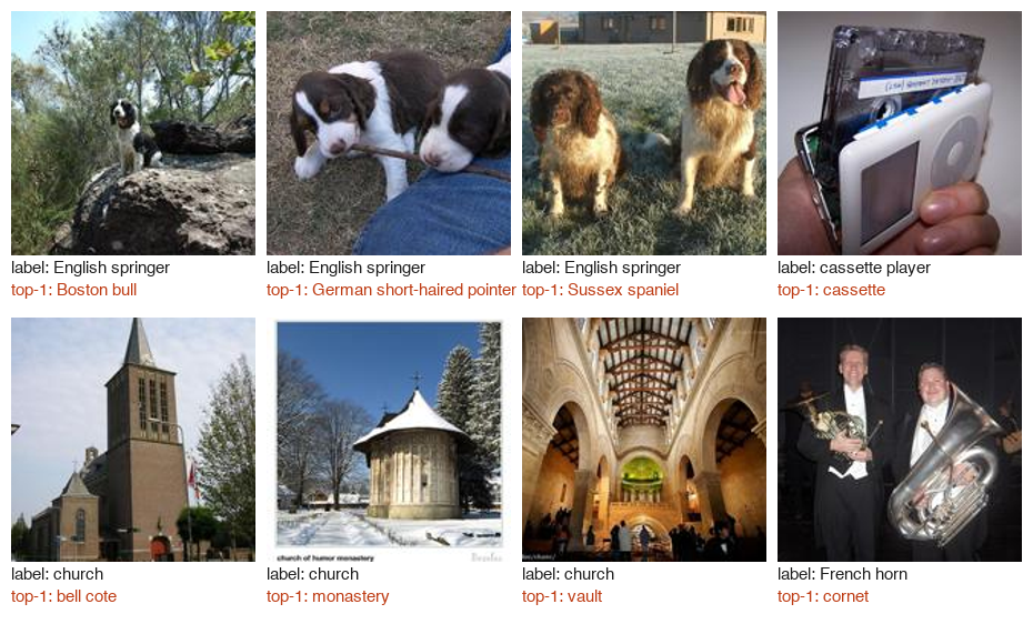
Top-5 forgives most mistakes: of ViT-L/16's 592 top-1 "errors", 499 have the correct label among its five best guesses. Are those real errors? Here are eight of them, picked at random:
plain text
  ViT-L/16, pictures whose top-1 is not the label but whose top-5 contains it (8 picked at random, seed 3):
    n02102040_2700.JPEG          label: English springer top-1: Boston bull            label at rank 3
    n02102040_8260.JPEG          label: English springer top-1: German short-haired pointer label at rank 3
    n02102040_880.JPEG           label: English springer top-1: Sussex spaniel         label at rank 2
    n02979186_15511.JPEG         label: cassette player  top-1: cassette               label at rank 2
    n03028079_26940.JPEG         label: church           top-1: bell cote              label at rank 2
    n03028079_9481.JPEG          label: church           top-1: monastery              label at rank 2
    n03028079_9560.JPEG          label: church           top-1: vault                  label at rank 3
    n03394916_38702.JPEG         label: French horn      top-1: cornet                 label at rank 2
Eight of ViT-L/16's top-1 "errors" on Imagenette, picked at random. The label is in black, the model's first answer in orange. In each case the correct label is the model's second or third answer.
Look at the pictures. The cassette is in the photo, inside the cassette player. A bell cote is the small tower that holds a church's bell, and the church photo shows one. The third church photo is taken inside, under its vault. The musicians hold a French horn and a second, larger brass instrument.
Only the three dog pictures are plain mistakes, and two of them name a similar hunting breed. Under ImageNet's single-label rule, all eight count as errors. Several of them are exactly what ReaL fixes.
So treat a single ImageNet number with care, especially near the top of the table. The ReaL paper found that part of the recent gains came from learning ImageNet's labelling habits. The ReaL row of Table 2 is the check on that, and ViT-H/14 still leads it (90.72%).
What this run cannot show: Imagenette's 10 classes are far easier than ImageNet's 1,000, and its pictures are stored at 160 pixels. Also, these ImageNet pictures may have been seen in pre-training. So the accuracies above are a lesson about the metrics, not a benchmark result.
Part 1 defined VTAB as 19 tasks with 1,000 training examples each. Here is what it set out to measure, in its own words:
The paper prints Figure 2 only as bars. Its Appendix D.10 (read at the end of this part) gives all 19 task scores for three ViT models. So we can recompute the ViT groups ourselves:
plain text
== 6. Table 9: the 19 VTAB-1k tasks, grouped as in Figure 2 ==
  ViT-H/14 (JFT)   mean of 19 = 77.63 (table: 77.6)   Natural 86.7   Specialized 87.0   Structured 65.0   lowest task: sNORB-Azim 33.2
  ViT-L/16 (JFT)   mean of 19 = 76.29 (table: 76.3)   Natural 85.6   Specialized 86.7   Structured 63.0   lowest task: sNORB-Azim 36.2
  ViT-L/16 (I21k)  mean of 19 = 72.71 (table: 72.7)   Natural 83.3   Specialized 84.7   Structured 57.5   lowest task: sNORB-Azim 30.5
Our ViT-H/14 values (86.7, 87.0 and 65.0) agree with the blue bars of Figure 2, as far as a bar chart can be read. The mean of the 19 tasks gives back Table 2's 77.63 exactly.
The 19 VTAB tasks of Table 9 averaged into Figure 2's groups, for the three ViT models of Table 2. Natural and Specialized tasks score in the 80s. Structured tasks are much harder (57.5 to 65.0) and gain the most from JFT-300M and a larger model.
Part 1 read two sentences of this section as the evidence behind "large scale training trumps inductive bias". Here is the whole section, with the experiments behind it.
Part 1 defined regularization. The three settings tuned here work in different ways:
A footnote on the same page explains one detail of the first series:
Appendix C holds the numbers behind Figure 3 (Table 5, read at the end of this part). Part 1 drew two of its models on ImageNet. Here are all five models and three of the six datasets:
Table 5 as three small charts, one per fine-tuning dataset. Each line is one ViT size across the three pre-training sets; dashed lines are the /32 models. On ImageNet, ViT-B/16 leads after ImageNet pre-training (77.91), and ViT-H/14 leads after JFT-300M (88.04). On CIFAR-100, the /32 models keep up with the /16 models.
The ranking of the five models on ImageNet changes with the data:
plain text
== 5. Table 5: ImageNet top-1 after fine-tuning, by pre-training dataset (the numbers behind Figure 3) ==
  pre-trained on ImageNet      ViT-B/16 77.91  ViT-B/32 73.38  ViT-L/16 76.53  ViT-L/32 71.16
      best to worst: ViT-B/16 > ViT-L/16 > ViT-B/32 > ViT-L/32;   ViT-L/16 - ViT-B/16 = -1.38
  pre-trained on ImageNet-21k  ViT-B/16 83.97  ViT-B/32 81.28  ViT-L/16 85.15  ViT-L/32 80.99  ViT-H/14 85.13
      best to worst: ViT-L/16 > ViT-H/14 > ViT-B/16 > ViT-B/32 > ViT-L/32;   ViT-L/16 - ViT-B/16 = +1.18
  pre-trained on JFT-300M      ViT-B/16 84.15  ViT-B/32 80.73  ViT-L/16 87.12  ViT-L/32 84.37  ViT-H/14 88.04
      best to worst: ViT-H/14 > ViT-L/16 > ViT-L/32 > ViT-B/16 > ViT-B/32;   ViT-L/16 - ViT-B/16 = +2.97
  ImageNet -> JFT-300M pre-training: ViT-B/16 gains +6.24 points, ViT-L/16 gains +10.59 points
Three things stand out. First, the winner changes. ViT-B/16 leads after ImageNet pre-training, and ViT-H/14 leads after JFT-300M. On ImageNet-21k the Huge model only ties ViT-L/16 (85.13 against 85.15), and the paper did not train it on ImageNet alone.
Second, more data helps the bigger model more: from ImageNet to JFT-300M, ViT-B/16 gains 6.24 points and ViT-L/16 gains 10.59. Third, ViT-L/32 jumps from last place to third. With a 32-pixel patch it has 4 times fewer tokens than ViT-L/16, so it sees the picture more coarsely. With enough data, its size starts to pay anyway.
The second series reports a "few-shot linear accuracy" instead of fine-tuning. Part 3 works the method out in full; here is what we need.
The idea: we want a weight matrix W that maps each representation x to a row of scores, one score per class. The target for a picture of class c is +1 at position c and −1 everywhere else (the paper's "{−1,1}K target vectors"). Least squares picks the W that makes the scores closest to the targets, with a penalty on large weights:
W=(X⊤X+λI)−1X⊤Y
Read it left to right. X is the n×d matrix of representations, one row per training picture (n=kK rows, d numbers each). Y is the n×K matrix of ±1 targets. X⊤X is d×d and measures how the features vary together. λI adds λ to its diagonal: the penalty on large weights, which also keeps the inverse well defined when n is small. X⊤Y is d×K and measures how each feature goes with each class.
A new picture gets the scores xW, and the largest score is the predicted class.
A tiny example, small enough for a pencil: four pictures with two features each, two classes, λ=1. The first two pictures are class 0, the last two class 1:
plain text
== 1. the few-shot closed form on a tiny example: 4 images, 2 features, 2 classes, lambda = 1 ==
  X (one row per image) = [[1.0, 0.0], [2.0, 1.0], [0.0, 2.0], [1.0, 3.0]]   classes [0, 0, 1, 1]
  Y (targets in {-1, 1}) = [[1.0, -1.0], [1.0, -1.0], [-1.0, 1.0], [-1.0, 1.0]]
  X^T X = [[6.0, 5.0], [5.0, 14.0]]   + lambda I = [[7.0, 5.0], [5.0, 15.0]]
  X^T Y = [[2.0, -2.0], [-4.0, 4.0]]
  W = (X^T X + I)^-1 X^T Y = [[0.625, -0.625], [-0.475, 0.475]]
  new image x = [1, 2]: scores x W = [-0.325, 0.325] -> class 1
Check one entry by hand. X⊤X has top-left entry 12+22+02+12=6; add λ=1 to get 7. The inverse of (75515) is 801(15−5−57), because 7⋅15−5⋅5=80. Its first row times the first column of X⊤Y, (2,−4), gives (15⋅2+5⋅4)/80=50/80=0.625. The new picture (1,2) scores 1⋅0.625+2⋅(−0.475)=−0.325 for class 0 and +0.325 for class 1, so it is class 1.
The tiny example as a picture. The class-0 pictures (squares) and class-1 pictures (circles) sit on either side of the line where both scores are equal. The new picture (1, 2) lands on the class-1 side.
Why use this instead of fine-tuning? One matrix inverse of size d×d replaces thousands of training steps. For ViT-L, d=1,024, so it is one 1,024×1,024 system of equations, tiny next to a training run. So the authors could score many checkpoints cheaply, and Figure 4 is made of these scores.
Section 4.3 in miniature: training from scratch on growing data#
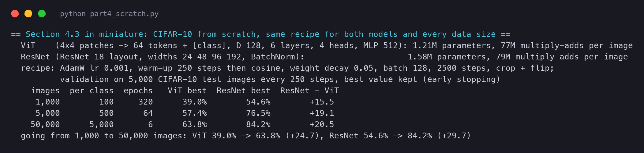
The paper's two series need hundreds of millions of pictures. We can still ask its question at a size a laptop can afford. We train both kinds of network from nothing, on more and more pictures, with one fixed recipe. The script vit_part4_scratch.py does it on CIFAR-10:
the data: random subsets of the 50,000 CIFAR-10 training pictures (1,000, 5,000 and all 50,000), each inside the next;
two models of matched cost: a small ViT from the same transformers code as the real one, and a small ResNet-18-style network. The ViT cuts the 32×32 picture into 4×4 patches, so it reads 64 patch tokens plus the class token;
one recipe for all six runs: AdamW, one learning-rate schedule, 2,500 steps of 128 pictures, random crops and flips. As in Section 4.3, early stopping keeps the best score on 5,000 held-out pictures.
plain text
== Section 4.3 in miniature: CIFAR-10 from scratch, same recipe for both models and every data size ==
  ViT    (4x4 patches -> 64 tokens + [class], D 128, 6 layers, 4 heads, MLP 512): 1.21M parameters, 77M multiply-adds per image
  ResNet (ResNet-18 layout, widths 24-48-96-192, BatchNorm):                     1.58M parameters, 79M multiply-adds per image
  recipe: AdamW lr 0.001, warm-up 250 steps then cosine, weight decay 0.05, batch 128, 2500 steps, crop + flip;
          validation on 5,000 CIFAR-10 test images every 250 steps, best value kept (early stopping)
    images  per class  epochs   ViT best  ResNet best  ResNet - ViT
     1,000        100     320      39.0%        54.6%        +15.5
     5,000        500      64      57.4%        76.5%        +19.1
    50,000      5,000       6      63.8%        84.2%        +20.5
  going from 1,000 to 50,000 images: ViT 39.0% -> 63.8% (+24.7), ResNet 54.6% -> 84.2% (+29.7)
The two models cost the same to run: 77 million and 79 million multiply-adds per picture. That matches the paper's pairing of "ViT-B/32" with "ResNet50" by speed rather than by size.
Best validation accuracy of the small ViT and the small ResNet, trained from scratch on 1,000, 5,000 and 50,000 CIFAR-10 pictures with one recipe. The ResNet is ahead at every size we can afford, by 15.5 to 20.5 points.
The ResNet wins at every size, by 15.5 to 20.5 points. This is the left edge of Figure 4, where the ResNets lead. Our largest set has 50,000 pictures. The paper's smallest subset has 9 million, 180 times more, and even there the ResNet-50 beats ViT-B/32. We are far below the region where the paper sees the lines cross.
The small ViT memorises. The training curves show what "overfit" means in practice:
plain text
== the training curves of vit_part4_scratch.py: validation accuracy (%) and smoothed training loss ==
   1,000 images  ViT    step 500: 36.0% / loss 1.272  step 1500: 37.7% / loss 0.080  step 2500: 38.6% / loss 0.004   best 39.0% at step 2000
   1,000 images  ResNet step 500: 47.5% / loss 0.360  step 1500: 53.3% / loss 0.003  step 2500: 54.1% / loss 0.001   best 54.6% at step 2000
  50,000 images  ViT    step 500: 41.5% / loss 1.657  step 1500: 57.7% / loss 1.230  step 2500: 63.8% / loss 1.059   best 63.8% at step 2500
  50,000 images  ResNet step 500: 55.0% / loss 1.047  step 1500: 79.7% / loss 0.594  step 2500: 84.2% / loss 0.432   best 84.2% at step 2500
With 1,000 pictures, both models drive the training loss to almost zero: they know every training picture by heart. But the ViT's validation accuracy stops near 38% to 39%, while the ResNet's reaches 54%. Both memorise; the ResNet's built-in assumptions make what it memorises more useful for new pictures. That is "the convolutional inductive bias is useful for smaller datasets", measured.
More data helps both, and the gap does not close here. From 1,000 to 50,000 pictures, the ViT gains 24.7 points and the ResNet 29.7. With 50,000 pictures, 2,500 steps are only 6 passes over the data, and both curves are still rising at the end. The fixed recipe now limits the result, and it limits the slower learner, the ViT, more. The paper does not say how many passes it made over each JFT subset. We could not afford longer runs on a shared laptop GPU.
What this experiment cannot show: the cross-over itself, which the paper finds between 9 million and 90 million pictures. Each point is one run, so differences of a point or two are noise. And CIFAR-10 pictures are 32×32, far from the 224×224 photos of JFT. What it does show is the starting point of the paper's story. At small scale, with the same recipe and the same cost, a ResNet beats a ViT clearly.
Few-shot on the released models: our small analogue of Figure 4#
We cannot pre-train on JFT subsets. But we can run Figure 4's measuring stick, the few-shot linear test, on models that Google released. The script vit_part4_fewshot.py freezes seven models and tests them on two datasets of Table 2:
the five ViT sizes of Figure 3 (B/32, B/16, L/32, L/16, H/14), all released after ImageNet-21k pre-training, with no fine-tuning;
two ResNet-50s as reference points: google/bit-50, a BiT R50x1 that ends in an ImageNet-1k head, and microsoft/resnet-50, trained on ImageNet-1k only;
CIFAR-100 (100 classes, 1,000 test pictures, 10 per class) and Oxford-IIIT Pets (37 breeds, 1,110 test pictures, 30 per class).
Every picture is resized to 224×224. For a ViT, the representation is its "pre-logits": the dense + tanh layer on the class token, which feeds the pre-training head. For a ResNet, it is the 2,048 pooled numbers.
For each k, we draw 5 random sets of k pictures per class from a pool of 20 per class. Each set gets the closed form above. The penalty λ is chosen once per model and dataset, from nine values, on 5 other training pictures per class. No test picture is ever used to choose anything.
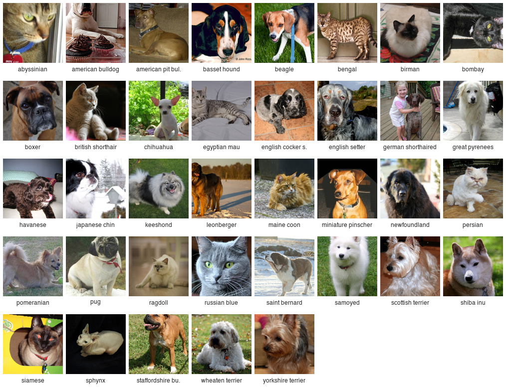
Here is what "1-shot" means on Pets: the whole training set of the first 1-shot draw, one picture per breed.
The complete training set of one 1-shot draw on Oxford-IIIT Pets: 37 pictures, one per breed. The frozen model never sees any other labelled picture of these breeds.
Our few-shot linear accuracy on frozen features, against labelled pictures per class (log scale). On CIFAR-100 every ViT pre-trained on ImageNet-21k is above both ResNet-50s at every k. On Pets the ResNet-50 trained on ImageNet-1k is on top at 10-shot (88.9%), and ViT-B/16 and the BiT ResNet share second place (87.6%).
First, few-shot works. With one picture of each of 100 classes, the frozen ViT-L/16 names 64.0% of CIFAR-100 test pictures correctly; chance is 1%. With 10 pictures per class it reaches 84.3%. For comparison, Table 2 reports 93.25% for the same kind of model after full fine-tuning on all 50,000 CIFAR-100 training pictures. Our number uses 1,000 labels and no training loop. That is the "very low-data transfer" of the paper's last paragraph.
Second, on CIFAR-100 the ImageNet-21k ViTs win clearly. At 10-shot, the five ViTs score 74.9% to 84.3%, the two ResNet-50s 69.4% and 56.1%. The closest to a fair pair is the one the paper names: "ViT-B/32 is slightly faster than ResNet50". Here ViT-B/32 scores 81.3% against 69.4% for the BiT ResNet. Two warnings: we cannot confirm which data google/bit-50 was pre-trained on, and microsoft/resnet-50 saw only 1.3 million pictures. So this is a comparison of released checkpoints, not of designs.
Third, Pets turns the order around, and the reason is the labels the models saw. At least 20 of the 37 Pets breeds are ImageNet-1k classes with the same name, such as "beagle", "pug" and "Persian cat". Both ResNet-50s were trained with exactly those labels, so their features already separate the breeds:
plain text
20 of 37 breeds have an ImageNet-1k class of the same name: american pit bull terrier, basset hound, beagle, boxer, chihuahua, english cocker spaniel, english setter, great pyrenees, keeshond, miniature pinscher, newfoundland, persian, pomeranian, pug, saint bernard, samoyed, scottish terrier, siamese, staffordshire bull terrier, yorkshire terrier
The ViTs saw ImageNet-21k's 21,000 classes, a much broader set that contains the ImageNet-1k classes among many others. The ImageNet-1k ResNet-50 is on top (88.9% at 10-shot), with ViT-B/16 (87.6%) and the BiT ResNet (87.6%) next. On CIFAR-100, whose classes are broad ones such as "apple", "cloud" or "bridge", the same ResNet-50 is last. A few-shot score measures how well the pre-training labels match the new task, as well as the model.
Fourth, bigger is not always better on ImageNet-21k. ViT-H/14 is below ViT-L/16 on both datasets (74.9% against 84.3% on CIFAR-100 at 10-shot). This matches the paper's own numbers for this pre-training set. In Table 5, after ImageNet-21k, ViT-H/14 only ties ViT-L/16 on ImageNet (85.13 against 85.15). The paper says that larger models show their full benefit "only with JFT-300M". Our run fits that pattern: 14 million pictures seem too few for a 632-million-parameter model.
We checked that our 16-bit arithmetic does not explain it. On four test pictures, ViT-H/14's features in 16-bit and 32-bit arithmetic point the same way:
plain text
== 4. does float16 change the features? ViT-H/14 on 4 CIFAR-100 test pictures, float16 on the GPU against float32 on the CPU ==
  cosine similarity float16 vs float32, per picture: 1.000000, 0.999999, 1.000000, 1.000000
A cosine similarity of 1 means the two feature vectors point in exactly the same direction. The ranking of the models is real for this protocol.
Fifth, the patch size matters less on CIFAR-100. ViT-B/32 (81.3%) is level with ViT-B/16 (80.6%) at 10-shot. The paper's Table 5 shows the same thing after ImageNet-21k pre-training: ViT-B/32 91.97 against ViT-B/16 91.67 on CIFAR-100. One likely reason: a CIFAR picture has only 32×32 real pixels, scaled up to 224, so a smaller patch finds no finer detail to read. That is our reading, not a claim of the paper.
What this experiment cannot show: it uses no JFT-300M, no fine-tuning and small test sets, and the checkpoints are not the paper's exact runs. The ± values are the spread over 5 draws of the training pictures (at k=10 they are below 1.3 points), not over test sets. The one thing it can show is the paper's practical point: a large pre-trained ViT gives useful features from a handful of labelled pictures.
== 4. Table 2 versus Table 5: ImageNet with and without Polyak averaging and 512/518 px fine-tuning ==
  ViT-H/14 (JFT)   Table 2: 88.55   Table 5 (384 px, no averaging): 88.04   difference +0.51
  ViT-L/16 (JFT)   Table 2: 87.76   Table 5 (384 px, no averaging): 87.12   difference +0.64
  ViT-L/16 (I21k)  Table 2: 85.30   Table 5 (384 px, no averaging): 85.15   difference +0.15
The two tricks are worth half a point for the JFT models, and 0.15 for the ImageNet-21k model. So part of the headline 88.55% is fine-tuning craft, not architecture. ViT-H/14 would still beat BiT-L's 87.54 without the tricks (88.04), but it would no longer pass Noisy Student's 88.4.
== 7. Table 7 (Appendix D.1): ResNets pre-trained on JFT with Adam or SGD, then fine-tuned ==
                       R50 Adam   R50 SGD  Adam-SGD  R152x2 Adam  R152x2 SGD  Adam-SGD
  ImageNet                77.54     78.24     -0.70        84.97       84.37     +0.60
  CIFAR10                 97.67     97.46     +0.21        99.06       99.07     -0.01
  CIFAR100                86.07     85.17     +0.90        92.05       91.06     +0.99
  Oxford-IIIT Pets        91.11     91.00     +0.11        95.37       94.79     +0.58
  Oxford Flowers-102      94.26     92.06     +2.20        98.62       99.32     -0.70
  average (ours)          89.33     88.79     +0.54        94.01       93.72     +0.29
  average (table)         89.33     88.79                  94.01       93.72
  Adam is higher in 7 of 10 dataset-model pairs
Our averages match the table to the last digit. One limit is worth stating: the test uses short pre-training (7 epochs). It shows that Adam is not a handicap in the paper's setting. It does not show that Adam beats SGD for ResNets in general.
Clevr-Count (count the objects in a synthetic scene) gains 21.4 points. Flowers102 gains 0.4, because it was already at 99.3. Bigger data and a bigger model mostly help where the task is far from photos of named objects. Note that these gaps mix two changes, the model size and the pre-training set, so they cannot be split between the two.
Next, in Part 5 (coming soon): Section 4.4 compares ViT, ResNets and hybrids at equal pre-training compute (Figure 5, Table 6). Then Section 4.5 opens the trained model: its patch filters, the position embeddings and how far its attention reaches, recomputed on the released weights. Last, Section 4.6 tries pre-training without labels. Part 5 is coming soon.
Run it yourself
Every number in this part that is not from the paper comes from the scripts in code/papers/vit/. vit_part4_tables.py runs no model; it recomputes the paper's tables. The other three download released checkpoints from Hugging Face. We ran them on an Apple M5 Pro GPU that other jobs shared, so we make no timing claims.
bash
pip install torch transformers pyarrow pillowpython vit_part4_tables.py # Table 2, 5, 7, 9 arithmetic and ObjectNet; no modelpython vit_part4_fewshot.py # the closed form by hand, then 7 frozen models on CIFAR-100 and Petspython vit_part4_top5.py # top-1 and top-5 of 4 ImageNet classifiers on Imagenettepython vit_part4_scratch.py # a small ViT and a small ResNet from scratch on CIFAR-10 subsetspython vit_part4_scratch_curves.py # prints the training curves saved by the run abovepython vit_part4_pictures.py # the 1-shot Pets picture
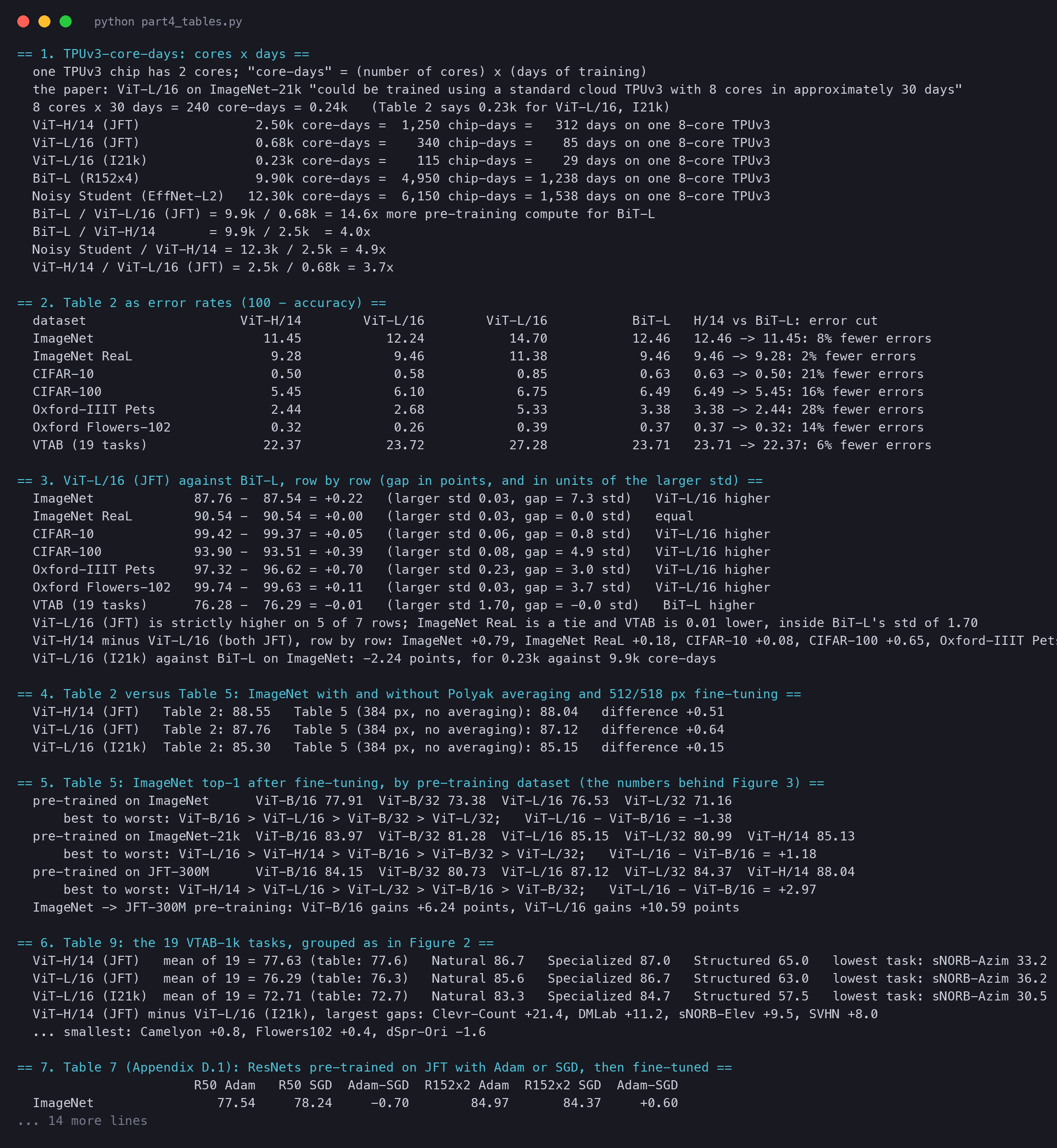
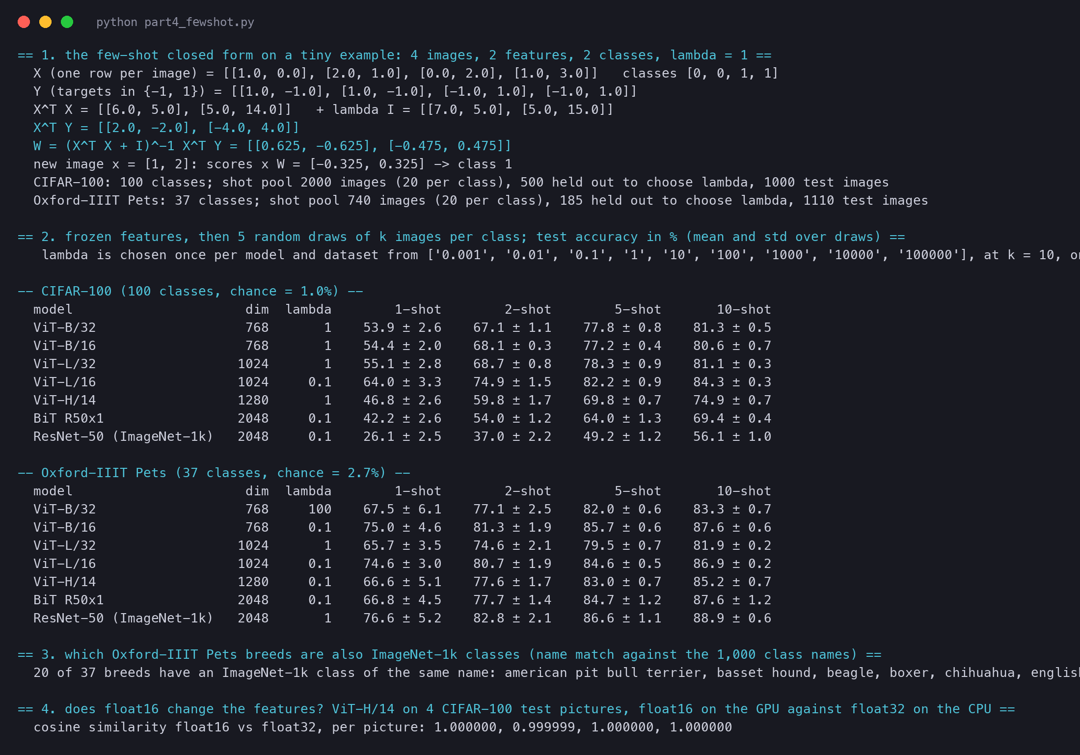
The real output of vit_part4_tables.py (first 60 lines).The real output of vit_part4_fewshot.py.The real output of vit_part4_scratch.py.