Transformer, explained · Part 5 of 7 · Covers §5, Eq. 3

Training: Data, Schedule, Adam and Regularization

How the Transformer was trained: the data, the batches, eight GPUs for twelve hours, Adam with a warm-up learning rate, dropout and label smoothing. We write each rule in Python, check it against PyTorch, and train a tiny Transformer step by step.

Attention Is All You Need. Ashish Vaswani, Noam Shazeer, Niki Parmar, Jakob Uszkoreit, Llion Jones, Aidan N. Gomez, Łukasz Kaiser, Illia Polosukhin. NeurIPS 2017, 2017. arXiv:1706.03762

A good network can still fail if you train it badly. Section 5 of the paper is one page long, and each line of it is a choice that made the Transformer train fast and well.

The training regime#

Parts 2 to 4 described the machine. This part describes how the machine learned. The section has four short pieces: the data, the hardware, the optimizer and the regularization. We read them in order.

The data#

The released model that we use in this series, Helsinki-NLP/opus-mt-en-de, has the paper's base shapes but a different vocabulary. It splits text with SentencePiece into 58,101 tokens. Our test sentence becomes these German pieces: ▁Matt + e for "Matte" (mat), and whole tokens for "Katze", "saß" and "müde". The ▁ sign marks the start of a word.

Batches of similar length#

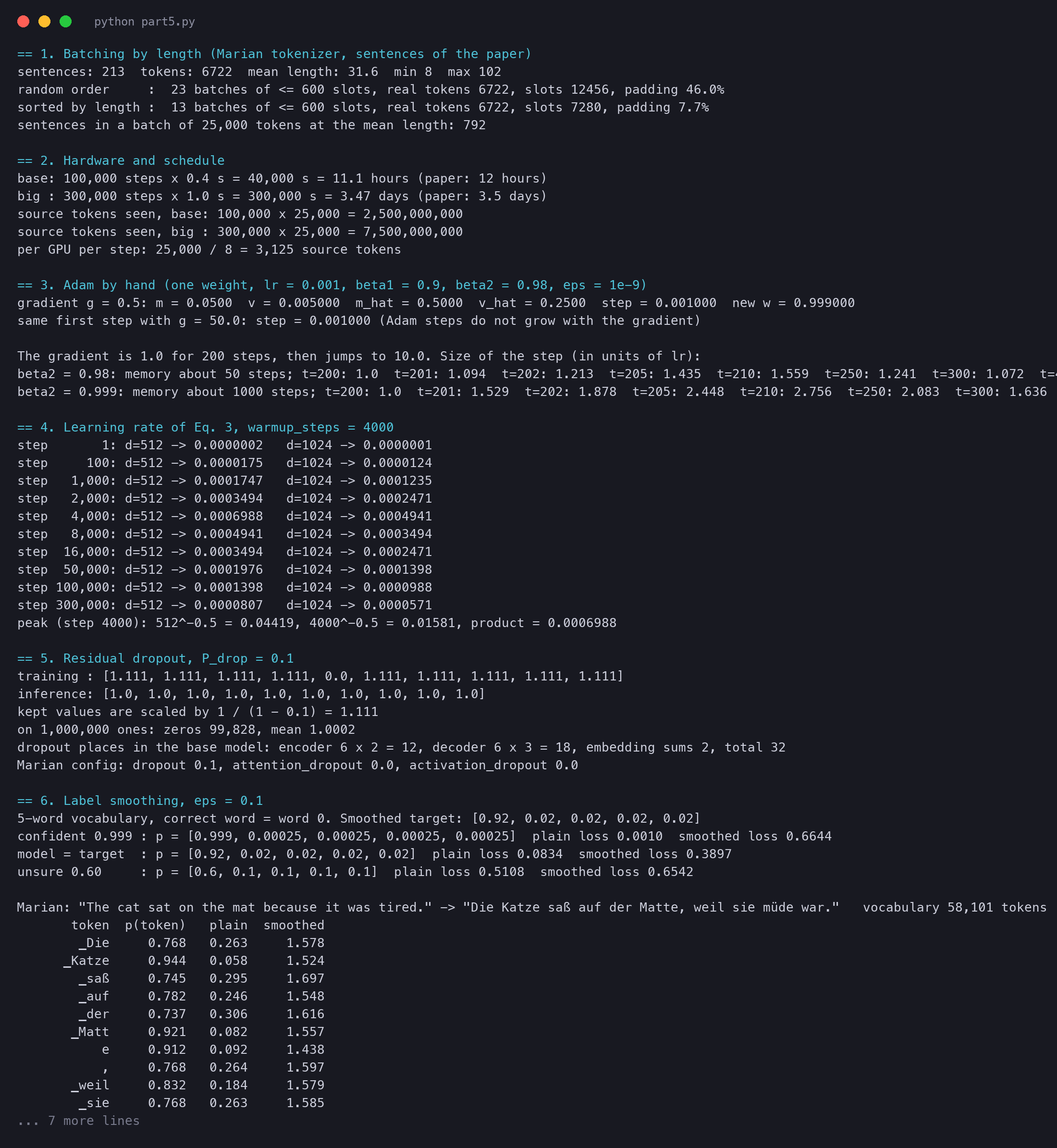
We tested this with the Marian tokenizer on the text of the paper itself. Its first ten pages give 213 sentences, with 6,722 tokens. A sentence has 31.6 tokens on average, from 8 to 102. We packed them into batches of at most 600 slots (rows × longest row), once in random order and once sorted by length.

random order     :  23 batches of <= 600 slots, real tokens 6722, slots 12456, padding 46.0%
sorted by length :  13 batches of <= 600 slots, real tokens 6722, slots 7280, padding 7.7%

In random order, almost half of the GPU's work is padding. Sorted by length, the waste falls to 7.7%, and the same text needs 13 batches instead of 23. At our mean length, a batch of 25,000 tokens would hold about 792 sentences. This is our own corpus and our own batch size. On WMT data the exact numbers will differ, but the gap will stay large.

Batching and padding masks in code#

Padding has a second problem, and it is worse than wasted work. Attention mixes every token with every other token. If the padding tokens take part, the output of a real word changes when you add padding next to it. So each batch carries a padding mask that tells the attention which positions to ignore.

Method 1: from scratch. The first function sorts the sentences by length and fills each batch until it would pass a budget of slots. The second function turns rows of different lengths into one rectangle and builds the mask at the same time.

def make_batches(token_lists, max_tokens):
    """Sort by length, then fill each batch until rows x longest row would pass max_tokens."""
    order = sorted(range(len(token_lists)), key=lambda i: len(token_lists[i]))
    batches, cur = [], []
    for i in order:
        longest = max(len(token_lists[j]) for j in cur + [i])
        if cur and longest * (len(cur) + 1) > max_tokens:
            batches.append(cur)
            cur = []
        cur.append(i)
    batches.append(cur)
    return batches


def pad_and_mask(rows, pad_id):
    """Rows of different lengths -> one rectangle of ids and a mask (1 = real token, 0 = padding)."""
    n = max(len(r) for r in rows)
    ids = torch.full((len(rows), n), pad_id)                   # (batch, n), all padding
    mask = torch.zeros((len(rows), n), dtype=torch.long)
    for i, r in enumerate(rows):
        ids[i, :len(r)] = torch.tensor(r)                         # real tokens on the left
        mask[i, :len(r)] = 1
    return ids, mask

We gave it eight sentences from the abstract and the introduction of the paper, with a budget of 48 slots per batch:

lengths in tokens: [7, 19, 9, 17, 8, 12, 22, 16]
batch of sentences [0, 4, 2, 5]: shape (4, 12), real tokens 36, padding 12
batch of sentences [7, 3]: shape (2, 17), real tokens 33, padding 1
batch of sentences [1, 6]: shape (2, 22), real tokens 41, padding 3
one batch of all 8 in the given order would hold 66 padding tokens; the sorted batches hold 16

The four short sentences travel together, and so do the two longest ones. The batch size in sentences changes from 4 to 2, but the size in slots stays near the budget. That is the paper's "25000 source tokens" rule at a small scale.

Method 2: with the library. The tokenizer can pad a list of sentences and build the mask itself. We padded the last batch both ways and compared the tensors:

last batch: our ids == tokenizer ids: True, our mask == tokenizer mask: True

Now the reason for the mask. We ran the Marian encoder on sentence 1 alone, and then inside its padded batch, with and without the mask. The first 19 output vectors should not depend on the 3 padding tokens after them.

with torch.no_grad():
    enc = model.get_encoder()
    alone = enc(input_ids=torch.tensor([ids_list[short]])).last_hidden_state[0]
    with_mask = enc(input_ids=ids, attention_mask=mask).last_hidden_state[k, :n_real]
    no_mask = enc(input_ids=ids).last_hidden_state[k, :n_real]

sentence 1 (19 tokens, padded to 22): encoder output alone vs in the batch
  with the padding mask   : max abs difference 1.4e-06
  without the padding mask: max abs difference 0.44

With the mask, the sentence gets the same vectors as when it is alone; 0.0000014 is rounding. Without the mask, the vectors change by up to 0.44, because the real words attend to the padding. A model trained like that would translate the same sentence differently in different batches.

Eight GPUs, twelve hours#

The "big" model is the bottom line of Table 3, which Part 6 covers. It has d_model = 1024 instead of 512, 16 heads instead of 8, and a feed-forward size of 4096. Each step is 2.5 times slower, and it trains 3 times longer.

The optimizer: Adam#

Here are the Adam rules for one weight θ with gradient g at step t:

Read it left to right. The first line keeps two running means: $m_t$ for the gradient and $v_t$ for its square. The numbers $\beta_1$ and $\beta_2$ say how much of the old average to keep at each step. Both averages start at 0, so they are too small at first; dividing by $1-\beta^t$ corrects this ("bias correction"). The update divides the mean by the root of the mean square. $\epsilon$ only guards against a division by zero.

A worked step. Take lr = 0.001, start from $m = v = 0$, and let the first gradient be $g = 0.5$. Then $m_1 = 0.1 \times 0.5 = 0.05$ and $v_1 = 0.02 \times 0.25 = 0.005$. Bias correction gives $\hat m = 0.05 / 0.1 = 0.5$ and $\hat v = 0.005 / 0.02 = 0.25$. The step is $0.001 \times 0.5 / \sqrt{0.25} = 0.001$. Our script prints the same:

gradient g = 0.5: m = 0.0500  v = 0.005000  m_hat = 0.5000  v_hat = 0.2500  step = 0.001000  new w = 0.999000
same first step with g = 50.0: step = 0.001000 (Adam steps do not grow with the gradient)

A gradient 100 times larger gives the same step. That is the point of Adam: the step size is set by the learning rate, not by the scale of the gradient.

Now β2. A running average with factor β remembers about $1/(1-\beta)$ steps. With 0.999, that is about 1,000 steps; with 0.98, about 50. We fed one weight a gradient of 1.0 for 200 steps, then a sudden jump to 10.0. We measured each step in units of the learning rate.

With 0.999, the mean of squares still remembers the small old gradients. So it is too small, and the step grows to almost three learning rates. With 0.98, the memory is short and the step stays near its normal size. In a Transformer, gradient sizes change fast early in training, so a short memory keeps the steps under control. The paper does not give this reason in words; this test shows the effect.

Adam in code#

Method 1: from scratch. Here is Adam as a small class. It keeps one $m$ and one $v$ for every weight, with the same shape as the weight. Each line of step is one line of the equations above.

class AdamByHand:
    """Adam, Section 5.3 of the paper, written out. One m and one v for every weight."""
    def __init__(self, params, lr=1e-3, beta1=0.9, beta2=0.98, eps=1e-9):
        self.params = list(params)
        self.lr, self.beta1, self.beta2, self.eps = lr, beta1, beta2, eps
        self.m = [torch.zeros_like(p) for p in self.params]   # running mean of the gradient
        self.v = [torch.zeros_like(p) for p in self.params]   # running mean of the squared gradient
        self.t = 0                                             # step counter

    @torch.no_grad()
    def step(self):
        self.t += 1
        for p, m, v in zip(self.params, self.m, self.v):
            g = p.grad
            m.mul_(self.beta1).add_((1 - self.beta1) * g)          # m = b1 m + (1 - b1) g
            v.mul_(self.beta2).add_((1 - self.beta2) * g * g)      # v = b2 v + (1 - b2) g^2
            m_hat = m / (1 - self.beta1 ** self.t)                 # bias correction: m and v start at 0
            v_hat = v / (1 - self.beta2 ** self.t)
            p -= self.lr * m_hat / (v_hat.sqrt() + self.eps)       # the step

The @torch.no_grad() line tells PyTorch that the update itself is not part of the model. The trailing underscore in mul_ and add_ means "change this tensor in place", so m and v keep their memory from step to step.

Method 2: with the library. PyTorch's Adam takes the paper's numbers as arguments: torch.optim.Adam(params, lr=1e-3, betas=(0.9, 0.98), eps=1e-9). We made two copies of one 4 × 3 weight matrix. Our class trained the first copy and PyTorch trained the second, on the same loss, for five steps.

A = nn.Parameter(W0.clone())             # copy 1, trained by our Adam
B = nn.Parameter(W0.clone())             # copy 2, trained by PyTorch's Adam
ours = AdamByHand([A], lr=1e-3)
lib = torch.optim.Adam([B], lr=1e-3, betas=(0.9, 0.98), eps=1e-9)
for t in range(1, 6):
    for P, o in ((A, ours), (B, lib)):
        P.grad = None
        loss = ((X @ P - Y) ** 2).mean()  # the same loss for both copies
        loss.backward()
        o.step()

step 1: loss 3.714999   max |A - B| = 0.0e+00   mean |change of a weight| = 0.001000
step 2: loss 3.708678   max |A - B| = 0.0e+00   mean |change of a weight| = 0.002000
step 3: loss 3.702367   max |A - B| = 0.0e+00   mean |change of a weight| = 0.003000
step 4: loss 3.696066   max |A - B| = 0.0e+00   mean |change of a weight| = 0.004000
step 5: loss 3.689773   max |A - B| = 0.0e+00   mean |change of a weight| = 0.004999

The two copies are identical to the last bit after every step. Look at the last column too. After step $t$, the mean change of a weight is $t \times 0.001$: one learning rate per step. The twelve weights have gradients of very different sizes, and Adam still gives them steps of the same size. That is the property of the worked example, now on a real matrix.

The warm-up schedule#

Here is Eq. 3 in standard notation, with $s$ for the step number and $w$ for the number of warm-up steps:

Read it from the right. The second term in the brackets, $s \cdot w^{-1.5}$, grows in a straight line with $s$. The first term, $s^{-0.5}$, falls with the step number. The min picks the smaller one, so the rate first rises with the line and then follows the falling curve. The two terms are equal at the peak, $s = w$, where both are $w^{-0.5}$. The factor $d_{\text{model}}^{-0.5}$ in front sets the overall height: a wider model gets a lower rate.

A worked example for the base model, $d_{\text{model}} = 512$ and $w = 4000$. The front factor is $512^{-0.5} = 0.04419$. At the peak, $4000^{-0.5} = 0.01581$, so the rate is $0.04419 \times 0.01581 = 0.000699$. At step 1,000, the line gives $1000 \times 4000^{-1.5} = 0.00395$, so the rate is $0.000175$, a quarter of the peak. At step 16,000, four times the peak step, the rate is $0.04419 \times 16000^{-0.5} = 0.000349$, half the peak.

step   1,000: d=512 -> 0.0001747   d=1024 -> 0.0001235
step   4,000: d=512 -> 0.0006988   d=1024 -> 0.0004941
step  16,000: d=512 -> 0.0003494   d=1024 -> 0.0002471
step 100,000: d=512 -> 0.0001398   d=1024 -> 0.0000988
step 300,000: d=512 -> 0.0000807   d=1024 -> 0.0000571

At the last step of the base run, step 100,000, the rate is 0.000140, one fifth of the peak. The big model never uses a higher rate than 0.000494, because its front factor is $1024^{-0.5} = 0.03125$. The paper does not say why it ties the rate to $d_{\text{model}}$. A fair reading: wider layers sum more numbers in each product. So the same change to each weight moves the output more, and a smaller rate balances that.

Warm-up became a standard part of Transformer training after this paper. Later work showed one main reason. In the paper's design, layer normalization comes after the residual sum ("post-norm", Part 2). Such networks can fail without warm-up. Moving the normalization before each sub-layer ("pre-norm") makes training less sensitive to it.

The schedule in code#

Method 1: from scratch. Eq. 3 is one line of Python. We split it into its two terms, so each name matches a part of the formula.

def lrate(step_num, d_model=512, warmup_steps=4000):
    """Eq. 3 of the paper. step_num starts at 1."""
    rise = step_num * warmup_steps ** -1.5      # straight line up during warm-up
    fall = step_num ** -0.5                     # 1 / sqrt(step) after warm-up
    return d_model ** -0.5 * min(rise, fall)    # the smaller of the two, scaled by the width

Method 2: with the library. PyTorch has a scheduler for any formula: LambdaLR. It multiplies the optimizer's learning rate by a function of the step. Two details make it match the paper. First, we give the optimizer lr=1.0, so the product is the value of our function. Second, LambdaLR counts from 0 and the paper counts from 1, so we shift by one.

# Method 2: PyTorch. LambdaLR multiplies the optimizer's lr by f(k), where k counts calls of
# scheduler.step() and starts at 0. So we set lr = 1.0 and shift k by one: f(k) = lrate(k + 1).
w = nn.Parameter(torch.zeros(1))
opt = torch.optim.Adam([w], lr=1.0, betas=(0.9, 0.98), eps=1e-9)
sched = torch.optim.lr_scheduler.LambdaLR(opt, lr_lambda=lambda k: lrate(k + 1))

worst = 0.0
for step_num in range(1, 20001):
    lib = opt.param_groups[0]['lr']             # the lr that this step uses
    ours = lrate(step_num)
    worst = max(worst, abs(lib - ours))
    if step_num in (1, 1000, 4000, 16000):
        log(f'step {step_num:>6,}: by hand {ours:.7f}   LambdaLR {lib:.7f}')
    opt.step()                                  # (no gradient here; only the schedule matters)
    sched.step()

step      1: by hand 0.0000002   LambdaLR 0.0000002
step  1,000: by hand 0.0001747   LambdaLR 0.0001747
step  4,000: by hand 0.0006988   LambdaLR 0.0006988
step 16,000: by hand 0.0003494   LambdaLR 0.0003494
max abs difference over 20,000 steps: 0.0e+00

The two agree at every one of the 20,000 steps. A common bug is to forget the shift. Then LambdaLR asks for step 0, and $0^{-0.5}$ is a division by zero. The order of the two calls matters too: opt.step() uses the current rate, and sched.step() then moves to the next one.

Regularization#

A large model can learn its training sentences by heart and then translate new sentences badly. This is overfitting. The paper uses "three types of regularization" against it. The page break splits the list: the two named types on page 8 are residual dropout and label smoothing.

Residual dropout#

We ran a PyTorch dropout layer with p = 0.1 on ten ones, and then on one million:

training : [1.111, 1.111, 1.111, 1.111, 0.0, 1.111, 1.111, 1.111, 1.111, 1.111]
inference: [1.0, 1.0, 1.0, 1.0, 1.0, 1.0, 1.0, 1.0, 1.0, 1.0]
on 1,000,000 ones: zeros 99,828, mean 1.0002

One of the ten ones became 0, and the other nine became 1/0.9 = 1.111. On a million values, 99,828 were dropped, about 10%, and the mean stayed at 1.0002. So the next layer sees the same average signal in training and at inference.

Method 1: from scratch. Dropout is three operations. Draw a random mask of 1s and 0s, multiply, and scale up what is left.

def dropout_by_hand(x, p=0.1, training=True):
    if not training:
        return x                                   # at inference dropout does nothing
    keep = torch.empty_like(x).bernoulli_(1 - p)   # 1 with probability 1 - p, else 0
    return x * keep * (1 / (1 - p))                # zero the dropped values, scale up the kept ones

bernoulli_(1 - p) is a coin toss for each number: it gives 1 with probability 0.9 and 0 with probability 0.1. The training flag is the switch that model.train() and model.eval() flip in a real network.

Method 2: with the library. nn.Dropout(0.1) draws its mask from the same random-number generator in the same way. So if we set the same seed before each call, the two masks should be the same, number for number. We tested it on 64 tokens of $d_{\text{model}} = 512$ random numbers:

same seed: max abs difference 0.0e+00; zeros 3301 of 32768 (10.07%)
mean of x -0.0131, mean after dropout -0.0129; inference: True

Our function and the library dropped the same 3,301 numbers and gave identical outputs. In inference mode both return the input unchanged ("True"). The mean moved only from −0.0131 to −0.0129, because the scale of 1/0.9 makes up for the dropped values.

Count the dropout places in the base model. Each of the 6 encoder layers has 2 sub-layers, so 12. Each of the 6 decoder layers has 3, so 18. Add the 2 embedding sums, and the total is 32. The released Marian model uses the same rate: its configuration has dropout 0.1, with no extra dropout inside attention or the feed-forward layer.

Label smoothing#

The smoothed target for token $k$, when the correct token is $y$ and the vocabulary has $V$ tokens, is:

Read it left to right. $[k = y]$ is 1 for the correct token and 0 for the others. So the correct token gets $1 - \epsilon$ plus its share of the spread, and every token gets $\epsilon / V$. The loss is the cross-entropy between this target $q$ and the model's prediction $p$. With $\epsilon = 0$ it is the normal loss, $-\log p_y$.

This is the form of the method's original paper. Some code spreads $\epsilon$ over the $V - 1$ wrong tokens only; for a large $V$ this changes almost nothing.

A tiny example with $V = 5$ words, where word 0 is correct. The target becomes $0.9 + 0.1/5 = 0.92$ for word 0, and $0.1/5 = 0.02$ for each other word.

Now compare three predictions. One is almost certain (0.999 on word 0), one equals the target, and one is unsure (0.6).

confident 0.999 : plain loss 0.0010  smoothed loss 0.6644
model = target  : plain loss 0.0834  smoothed loss 0.3897
unsure 0.60     : plain loss 0.5108  smoothed loss 0.6542

The normal loss loves the confident prediction: 0.0010. The smoothed loss punishes it: 0.6644, worse than the unsure one. The lowest smoothed loss, 0.3897, is at the target itself. That is the whole effect in three lines: the model is pulled toward 92%, not toward 100%.

We ran the same test on the released Marian model. It translated "The cat sat on the mat because it was tired." as "Die Katze saß auf der Matte, weil sie müde war." We then measured its probability for each token of that translation.

       token  p(token)   plain  smoothed
        ▁Die     0.768   0.263     1.578
      ▁Katze     0.944   0.058     1.524
       ▁müde     0.834   0.182     1.568
mean plain loss 0.184 (perplexity 1.20),  mean smoothed loss 1.545
lowest possible smoothed loss with 58,101 tokens (prediction = target): 1.422; each other token gets 1.72e-06

The model gives its chosen tokens 0.834 on average, never close to 1. The smoothed loss looks large, 1.545, but even a perfect prediction cannot go below 1.422 here. The reason is the spread: each of the 58,100 other tokens should get 0.1/58,101 = 0.0000017, and that costs about 1.33 alone. We did not check how Marian was trained. So this test shows the size of the two losses, not the effect of smoothing on this model. The perplexity of 1.20 is on the model's own output, which is an easy test; the paper's perplexities in Part 6 are on human translations.

Label smoothing in code#

The paper's sentence, "label smoothing of value ϵls = 0.1", does not say where the 0.1 goes. There are two common answers, and they give different targets. PyTorch gives $\epsilon / V$ to every token, the correct one too, as in the formula above. Other code, the paper's own tensor2tensor library among them, gives $1 - \epsilon$ to the correct token and $\epsilon / (V - 1)$ to each wrong one. We write both.

Method 1: from scratch. The first function builds the target $q$. The second takes the log-softmax of the logits and computes the cross-entropy with $q$. It can also skip padding positions, as a real training loop must.

def smoothed_targets(y, V, eps=0.1, spread_over='all'):
    """The target distribution q for each position. y: (n,) correct token ids."""
    n = y.shape[0]
    if spread_over == 'all':                 # eps / V to every token, the correct one too (PyTorch, Szegedy et al.)
        q = torch.full((n, V), eps / V)
        q[torch.arange(n), y] += 1 - eps
    else:                                    # eps / (V - 1) to the wrong tokens only
        q = torch.full((n, V), eps / (V - 1))
        q[torch.arange(n), y] = 1 - eps
    return q


def smoothed_loss_by_hand(logits, y, eps=0.1, spread_over='all', ignore_index=None):
    log_p = torch.log_softmax(logits, dim=-1)              # (n, V) log probabilities
    q = smoothed_targets(y.clamp(min=0), logits.shape[-1], eps, spread_over)
    per_position = -(q * log_p).sum(-1)                   # cross-entropy between q and p
    if ignore_index is not None:                          # padding positions do not count
        keep = y != ignore_index
        return per_position[keep].mean()
    return per_position.mean()

Method 2: with the library. nn.CrossEntropyLoss(label_smoothing=0.1) does all of this in one call, and ignore_index names the padding token. We compared the two on our five-word example, on a batch with padding, and on the real Marian logits from above:

5 words, logits [4.0, 0.5, 0.0, -0.5, 0.2], correct word 0, p = [0.9242, 0.0279, 0.0169, 0.0103, 0.0207]
target, eps over all 5 words     : [0.92, 0.02, 0.02, 0.02, 0.02]
target, eps over the 4 wrong ones: [0.9, 0.025, 0.025, 0.025, 0.025]
loss by hand 0.394805   CrossEntropyLoss 0.394805   difference 0.0e+00
loss with eps over the wrong words only: 0.473805
24 positions (6 of them padding), V = 1,000: by hand 11.374208   library 11.374207   difference 1.9e-06
Marian, 14 target tokens, V = 58,101: by hand 1.545421   library 1.545421   eps over the wrong tokens only 1.545445

Our loss equals the library's in all three cases; the 0.0000019 on the padded batch is rounding. On the Marian sentence, both give 1.545, the number of the table above.

With five words, the two readings of the paper differ clearly. One target is 0.92 for the correct word and the other is 0.90, and the losses are 0.395 and 0.474. With 58,101 tokens, the difference almost vanishes: 1.545421 against 1.545445. The share of each wrong token changes from $0.1/58{,}101$ to $0.1/58{,}100$, which is no real change. So for a translation vocabulary, you can use PyTorch's version and still follow the paper. For a small vocabulary, choose on purpose and say which one you use.

One training step, written out#

Section 5 lists its rules one by one. A training program uses them all at once, in a fixed order, many thousands of times. Here is that order on a tiny Transformer that we trained on the CPU. Its task: read a list of 3 to 8 digits and write it backwards. Lists of different lengths need padding, so every rule of this page takes part.

The model is PyTorch's own nn.Transformer, which has the paper's post-norm layers, with our embeddings and sine-wave positions around it. (Part 7 builds the whole network from scratch; here the subject is the training loop.)

class TinyTransformer(nn.Module):
    """Embeddings + sinusoidal positions + nn.Transformer (post-norm, as in the paper) + an output layer."""
    def __init__(self, small_init=True):
        super().__init__()
        self.emb = nn.Embedding(V, D_MODEL, padding_idx=PAD_ID)
        if small_init:                        # small start, so x sqrt(d_model) gives about 1
            nn.init.normal_(self.emb.weight, std=D_MODEL ** -0.5)
        pos = torch.arange(32)[:, None]
        i = torch.arange(0, D_MODEL, 2)
        pe = torch.zeros(32, D_MODEL)
        pe[:, 0::2] = torch.sin(pos / 10000 ** (i / D_MODEL))
        pe[:, 1::2] = torch.cos(pos / 10000 ** (i / D_MODEL))
        self.register_buffer('pe', pe)
        self.drop = nn.Dropout(0.1)
        self.core = nn.Transformer(D_MODEL, HEADS, LAYERS, LAYERS, D_FF, dropout=0.1, batch_first=True)
        self.out = nn.Linear(D_MODEL, V)

    def embed(self, ids):                     # token embedding * sqrt(d_model) + position, then dropout
        return self.drop(self.emb(ids) * D_MODEL ** 0.5 + self.pe[:ids.shape[1]])

    def forward(self, src, tgt_in):
        m = tgt_in.shape[1]
        causal = torch.triu(torch.ones(m, m, dtype=torch.bool), diagonal=1)   # True = may not look (future)
        h = self.core(self.embed(src), self.embed(tgt_in), tgt_mask=causal, tgt_is_causal=True,
                      src_key_padding_mask=src == PAD_ID, tgt_key_padding_mask=tgt_in == PAD_ID,
                      memory_key_padding_mask=src == PAD_ID)
        return self.out(h)                    # (batch, m, V) scores for the next token

Three masks go into self.core. The causal mask stops the decoder from looking at future tokens (Part 3). The two padding masks stop all attention from looking at padding. Dropout acts on the embedding sums here, and nn.Transformer applies it to each sub-layer output, as §5.4 asks.

The small_init switch in __init__ taught us a lesson; the result is at the end of this section.

The paper does not mention gradient clipping. We add it because most training programs today use it, and it shows where such a guard goes. First we checked our own version against PyTorch's clip_grad_norm_:

def clip_by_hand(params, max_norm):
    """What clip_grad_norm_ does: one norm over all gradients, then one scale factor for all."""
    grads = [p.grad for p in params if p.grad is not None]
    total = torch.sqrt(sum((g ** 2).sum() for g in grads))
    scale = min(1.0, max_norm / (total.item() + 1e-6))
    return total, [g * scale for g in grads]

tiny model: d_model 64, 4 heads, d_ff 128, 2+2 layers, 169,357 weights
gradient norm by hand 1.6337, clip_grad_norm_ 1.6337; clipped gradients max abs difference 0.0e+00

Now the step itself. Each numbered comment is one stage, and the order matters.

def train_step(model, batch, opt, sched, loss_fn, max_norm=1.0):
    src, tgt_in, tgt_out = batch
    model.train()                                              # dropout on
    logits = model(src, tgt_in)                                # 1. forward pass      (batch, m, V)
    loss = loss_fn(logits.reshape(-1, V), tgt_out.reshape(-1)) # 2. loss, smoothed, padding ignored
    opt.zero_grad()                                            # 3. forget the old gradients
    loss.backward()                                            # 4. backward pass: new gradients
    norm = nn.utils.clip_grad_norm_(model.parameters(), max_norm)  # 5. clip the gradient norm
    opt.step()                                                 # 6. Adam changes every weight
    sched.step()                                               # 7. next learning rate of Eq. 3
    return loss.item(), norm.item()

Read it as a story. The model makes its guesses (1), and the loss grades them against the smoothed targets (2). PyTorch adds new gradients to old ones, so we clear the old ones first (3). The backward pass computes the new gradients (4), and clipping limits their total length (5). Adam moves every weight (6), and the schedule sets the rate for the next step (7). If you swap 5 and 6, the clip comes too late; if you forget 3, each step uses the sum of all past gradients.

The batch gives the decoder the target shifted right by one. The decoder reads the start token and the first $k$ digits, and it must predict digit $k + 1$. This is "teacher forcing" from Part 1: during training, the decoder always sees the correct past, not its own guesses.

def make_batch(n_rows, gen):
    """Random digit lists of length 3 to 8; the target is the list reversed. Padded, with BOS and EOS."""
    lens = torch.randint(3, 9, (n_rows,), generator=gen)
    rows = [torch.randint(3, 13, (int(L),), generator=gen) for L in lens]
    src, _ = pad_and_mask([r.tolist() + [EOS] for r in rows], PAD_ID)
    tgt, _ = pad_and_mask([[BOS] + r.flip(0).tolist() + [EOS] for r in rows], PAD_ID)
    return src, tgt[:, :-1], tgt[:, 1:]      # decoder input is the target shifted right by one

Everything else comes from the earlier sections: the paper's Adam, Eq. 3 through LambdaLR with 200 warm-up steps, and label smoothing that ignores padding.

opt = torch.optim.Adam(model_t.parameters(), lr=1.0, betas=(0.9, 0.98), eps=1e-9)
sched = torch.optim.lr_scheduler.LambdaLR(opt, lambda k: lrate(k + 1, D_MODEL, WARMUP))
loss_fn = nn.CrossEntropyLoss(label_smoothing=0.1, ignore_index=PAD_ID)

We ran 1,000 steps of 64 lists each:

step    1: lr 0.00004   loss 2.640   gradient norm before clipping 1.44
step   50: lr 0.00221   loss 1.778   gradient norm before clipping 0.89
step  100: lr 0.00442   loss 1.232   gradient norm before clipping 1.46
step  200: lr 0.00884   loss 0.937   gradient norm before clipping 1.44
step  400: lr 0.00625   loss 0.726   gradient norm before clipping 1.52
step  600: lr 0.00510   loss 0.708   gradient norm before clipping 1.91
step 1000: lr 0.00395   loss 0.598   gradient norm before clipping 2.24
lowest possible smoothed loss with V = 13: 0.537
1000 steps in 26 s on the CPU
example: [5, 4, 9, 5, 6, 1] -> [1, 6, 5, 9, 4, 5]
exact reversals on 500 new lists: 491 / 500

The learning rate climbs to its peak at step 200 and then falls, as Eq. 3 says. The loss falls from 2.640 toward 0.598. It can never reach 0, because of label smoothing: with 13 tokens, the floor is 0.537. On 500 new lists that the model never saw, it wrote 491 exactly backwards. Our tiny model has $d_{\text{model}} = 64$, so its peak rate, 0.00884, is much higher than the base model's 0.000699. The factor $d_{\text{model}}^{-0.5}$ of Eq. 3 does that on its own.

Now the lesson of small_init. The paper multiplies each embedding by $\sqrt{d_{\text{model}}}$, here 8, before it adds the position code. PyTorch starts an embedding with a spread of 1. After the factor 8, the token vectors are about 8 times larger than the position codes. We trained the same model again on the same batches, but with that default start:

same run, embeddings started with spread 1 (PyTorch default): loss 1.160, exact reversals 144 / 500

Only 144 of 500 lists came out right, against 491. The model hardly saw the positions, and reversal is a task about positions. With a starting spread of $d_{\text{model}}^{-0.5}$, the product is about 1, the same size as the sines and cosines. The paper names the factor $\sqrt{d_{\text{model}}}$ in §3.4 but not the starting spread. The two only work as a pair.

What these choices bought#

None of these rules is new on its own. Adam, dropout, label smoothing and length-sorted batches all existed before 2017. The new parts are the warm-up schedule tied to $d_{\text{model}}$, and a recipe that worked for a network with no recurrence. Part 6 shows the result. The base model beat most earlier systems after 12 hours, and Table 3 tests other values of dropout and label smoothing.

What our tests cannot show: we did not train a full-size Transformer here. Our tiny model learns a toy task in 26 seconds; WMT needs the paper's 12 hours on 8 GPUs. The batching test uses the paper's own text, not WMT data. The Adam test uses one weight with a made-up gradient. The Marian model has the base shapes, but its data, vocabulary and training settings are not the paper's.

The code of the sections "in code" is in tx_part5_code.py, and its full output is in results/part5_code_stdout.txt. It runs on a laptop CPU in under a minute.

The paper and the code#

Paper (arXiv 1706.03762) · Official code (tensor2tensor) · Our scripts for this series