Transformer, explained · Part 6 of 7 · Covers §6.1, Table 2, §6.2, Table 3, §6.3, Table 4, §7, Figures 3 to 5
Results, Variations and Impact
What the Transformer scored, what it cost to train, which parts of it matter, and how it did on a second task. We write BLEU, beam search, checkpoint averaging and the size count in Python, and check each one against a library.
Attention Is All You Need. Ashish Vaswani, Noam Shazeer, Niki Parmar, Jakob Uszkoreit, Llion Jones, Aidan N. Gomez, Łukasz Kaiser, Illia Polosukhin. NeurIPS 2017, 2017. arXiv:1706.03762
The first five parts built the Transformer and trained it. This part asks two questions: how well does it work, and what does it cost?
Translation results
The paper measures translation quality with one number, BLEU. Every result below uses it, so we start there.
Think of BLEU as a teacher who grades a translation with a highlighter. The teacher has the human translation beside the student's text. She marks every single word that also appears in the human text. Then she marks every pair of words, every group of three and every group of four. Long matches are hard to get by luck, so they show that the word order is right too.
Read it from left to right:
- is the precision for groups of words: the fraction of the output's -word groups that also appear in the human translation.
- The sum of inside is the geometric mean of the four precisions. If any one of them is very low, the score falls.
- is the brevity penalty. is the length of the output and the length of the human translation. An output that is too short loses points, because a short output can reach high precision by saying almost nothing.
- The result is multiplied by 100 for the tables.
A tiny example. The human text is "the cat sat on the mat" and the machine writes "the cat sat on a mat". Count the matches:
| group size | groups in the output | groups that match | |
|---|---|---|---|
| 1 | 6 | 5 (all but "a") | 5/6 = 0.833 |
| 2 | 5 | 3 ("the cat", "cat sat", "sat on") | 3/5 = 0.600 |
| 3 | 4 | 2 ("the cat sat", "cat sat on") | 2/4 = 0.500 |
| 4 | 3 | 1 ("the cat sat on") | 1/3 = 0.333 |
Both texts have 6 words, so . The geometric mean is . The score is 53.7. One wrong word took away almost half of the points, because it broke three of the longer groups. Real scores are computed over a whole test set of about 3,000 sentences, not one sentence.
BLEU in code
Method 1: from scratch. BLEU needs four small functions. The first counts word groups. The second compares one output with its reference. The third turns the counts into a score, and the fourth does it for a whole test set.
def ngrams(words, n):
    """Count every group of n words that follow each other."""
    return Counter(tuple(words[i:i + n]) for i in range(len(words) - n + 1))


def bleu_stats(hyp, ref, max_n=4):
    """For one sentence: matches and totals for n = 1..4, and the two lengths."""
    hyp, ref = hyp.split(), ref.split()
    matches, totals = [], []
    for n in range(1, max_n + 1):
        h, r = ngrams(hyp, n), ngrams(ref, n)
        # clipping: a group counts at most as often as it occurs in the reference
        matches.append(sum(min(count, r[g]) for g, count in h.items()))
        totals.append(max(len(hyp) - n + 1, 0))
    return matches, totals, len(hyp), len(ref)


def bleu_from_stats(matches, totals, c, r):
    if min(matches) == 0:
        return 0.0                                   # log(0): one empty precision makes the score 0
    log_mean = sum(math.log(m / t) for m, t in zip(matches, totals)) / len(matches)   # geometric mean, in logs
    bp = 1.0 if c > r else math.exp(1 - r / c)       # brevity penalty: only short outputs lose points
    return 100 * bp * math.exp(log_mean)


def corpus_bleu(hyps, refs):
    """Corpus BLEU adds up the counts of all sentences first, then computes one score."""
    M, T, C, Rl = [0] * 4, [0] * 4, 0, 0
    for h, r in zip(hyps, refs):
        m, t, c, rl = bleu_stats(h, r)
        M = [a + b for a, b in zip(M, m)]
        T = [a + b for a, b in zip(T, t)]
        C, Rl = C + c, Rl + rl
    return bleu_from_stats(M, T, C, Rl)
Read ngrams first. For "the cat sat" and it slides a window of two words along the sentence and counts ("the", "cat") and ("cat", "sat"). A Counter is a dictionary that counts, so a group that occurs twice gets the value 2.
bleu_stats holds the one idea of BLEU that the formula hides: clipping. Without it, the output "the the the the the the" would have six matching words, because "the" is in the reference. With clipping, "the" counts at most as often as the reference has it, which is twice. The line min(count, r[g]) does this. totals is the number of groups in the output. A sentence of 6 words has 6 single words, 5 pairs, 4 triples and 3 groups of four.
bleu_from_stats follows the formula. It takes the mean of the four log precisions, which is the log of their geometric mean. The brevity penalty is 1 when the output is longer than the reference, and when it is shorter. If any precision is 0, its log is minus infinity and the score is 0.
Method 2: with the library. The standard tool is sacreBLEU. It fixes the tokenization and the details, so that teams can compare scores. It is not in our Python environment, so we installed it into a separate folder only for this check. We ran both on four outputs against "the cat sat on the mat":
sacrebleu: 2.6.0
"the cat sat on a mat": p1..p4 = 5/6 3/5 2/4 1/3, c = 6, r = 6, BLEU ours 53.73, sacrebleu 53.73
"the cat sat on the mat": p1..p4 = 6/6 5/5 4/4 3/3, c = 6, r = 6, BLEU ours 100.00, sacrebleu 100.00
"the cat sat on": p1..p4 = 4/4 3/3 2/2 1/1, c = 4, r = 6, BLEU ours 60.65, sacrebleu 60.65
"the the the the the the": p1..p4 = 2/6 0/5 0/4 0/3, c = 6, r = 6, BLEU ours 0.00, sacrebleu 0.00
sacrebleu with its default smoothing on the last one: 9.65
unclipped: "the" counted 6 times; clipped: min(6, 2) = 2
two sentences: sentence BLEU 53.73 and 41.11 (mean 47.42); corpus BLEU ours 46.27, sacrebleu 46.27
Our 53.73 is the 53.7 of the table above, and sacreBLEU agrees on every line. The third output shows the brevity penalty at work. "the cat sat on" has perfect precisions, but it has 4 words where the reference has 6. So , and the score is 60.65, not 100. The fourth output gets only 2 matches out of 6 words after clipping, and no matching pairs, so its score is 0.
Two details matter for real use. First, sacreBLEU's sentence_bleu smooths empty precisions by default, so the hopeless fourth output gets 9.65 instead of 0. We turned that smoothing off for the comparison. Second, corpus BLEU is not the mean of the sentence scores. It adds up the matches and totals of all sentences, then computes one score: 46.27 for our two sentences, not their mean of 47.42. The scores in the paper's tables are corpus scores of this kind.
How the training cost was counted
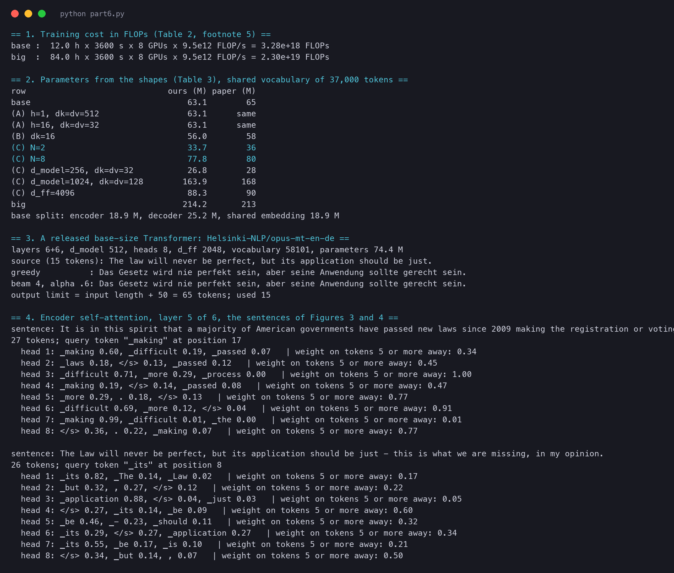
Here is the training time in seconds, the number of cards, and the speed of one card in operations per second. Part 5 gave the times: 12 hours for the base model and 3.5 days for the big model, both on 8 P100 cards. Our script does the multiplication:
base :  12.0 h x 3600 s x 8 GPUs x 9.5e12 FLOP/s = 3.28e+18 FLOPs
big  :  84.0 h x 3600 s x 8 GPUs x 9.5e12 FLOP/s = 2.30e+19 FLOPs
Both numbers match Table 2: and . The big model costs 7 times as much as the base model: 3 times the steps, and each step more than twice as slow.
Averaged checkpoints and beam search
Beam search compares sentences by their log probability: the sum of the logs of the probability of each word. Each word adds a negative number, so a long sentence always has a lower score than a short one. Without a fix, beam search prefers short translations. The length penalty from the GNMT paper divides the score by a factor that grows with the length :
Here is the source sentence, a candidate translation, and sets the strength of the penalty. With there is no correction. A tiny example with : a short candidate of 4 tokens has , and a long one of 8 tokens has . The factors are and . The scores become and . The long candidate now wins, although its raw log probability was lower.
We ran a released translator with these settings. Helsinki-NLP/opus-mt-en-de is a Marian model with the paper's base shapes: 6 + 6 layers, , 8 heads, and sinusoidal positions. It was trained on other data with another vocabulary, so it is not the paper's model.
layers 6+6, d_model 512, heads 8, d_ff 2048, vocabulary 58101, parameters 74.4 M
source (15 tokens): The law will never be perfect, but its application should be just.
greedy          : Das Gesetz wird nie perfekt sein, aber seine Anwendung sollte gerecht sein.
beam 4, alpha .6: Das Gesetz wird nie perfekt sein, aber seine Anwendung sollte gerecht sein.
output limit = input length + 50 = 65 tokens; used 15
For this sentence, greedy decoding and beam search give the same correct German. That is common for short, clear sentences. Beam search helps on hard sentences, where the best first word is not the best start for the whole sentence. We do not measure BLEU on the model here: we have no WMT test set, so any score from us would be a guess.
Checkpoint averaging in code
Checkpoint averaging is the shortest algorithm on this page. A checkpoint is a dictionary from weight names to tensors, so the average is one dictionary of means.
Method 1: from scratch.
def average_by_hand(state_dicts):
    """Weight by weight: the mean of the same tensor over all checkpoints."""
    return {k: sum(sd[k] for sd in state_dicts) / len(state_dicts) for k in state_dicts[0]}
To see it work, we need weights that still move at the end of training. We trained a tiny network (8 inputs, 32 hidden units, 1 output) on a noisy curve, with plain gradient descent and a large step. We saved a checkpoint every 100 steps, our stand-in for the paper's "10-minute intervals", and averaged the last 5.
Method 2: with the library. PyTorch has torch.optim.swa_utils.AveragedModel, which keeps a running mean of the weights it is given. "SWA" means stochastic weight averaging, a later method built on the same idea.
last5 = checkpoints[-5:]
avg = average_by_hand(last5)
swa = AveragedModel(net)                  # Method 2: the library keeps a running mean
for sd in last5:
    net.load_state_dict(sd)
swa.update_parameters(net)one weight in the last 5 checkpoints: -0.4073, -0.3782, -0.4102, -0.4517, -0.4189 -> mean -0.4133
validation loss of the last 5 checkpoints: 0.8701, 0.9201, 0.9074, 0.8006, 0.8326
validation loss of their average: 0.7449
average by hand vs AveragedModel: max abs difference 1.2e-07The first line is the needle of the scale from the box above. One weight jumps between −0.45 and −0.38, and the average sits in the middle. The validation loss is measured on new data that the network never trained on. Every single checkpoint scores between 0.80 and 0.92, and their average scores 0.7449, better than all five. The noise of the last steps pushes each checkpoint a little off in a random direction, and the average cancels much of it. The library's running mean agrees with ours to 0.00000012, which is rounding.
One condition hides in this trick. The five checkpoints must be close to each other, in the same valley of the loss. Averaging two networks trained from different random starts usually gives a poor network, because their hidden units can be in a different order. The paper averages checkpoints only 10 minutes apart, so the condition holds.
Greedy decoding in code
model.generate hides the decoding loop. Here we write it ourselves around the released Marian model. We use the model only for one thing: given the source and the tokens so far, give the log probability of every possible next token.
@torch.no_grad()
def encode(text):
    x = tok([text], return_tensors='pt')
    memory = model.get_encoder()(**x).last_hidden_state     # (1, n, 512), computed once
    return x, memory


@torch.no_grad()
def next_log_probs(x, memory, prefixes):
    """log P(next token | source, prefix) for each prefix. prefixes: (beams, t) -> (beams, V)."""
    b = prefixes.shape[0]
    out = model(encoder_outputs=BaseModelOutput(last_hidden_state=memory.expand(b, -1, -1)),
                attention_mask=x['attention_mask'].expand(b, -1), decoder_input_ids=prefixes)
    logits = out.logits[:, -1]                    # scores for the token after the prefix
    logits[:, PAD] = -float('inf')                # the padding token is never a word
    return torch.log_softmax(logits, dim=-1)
The encoder runs once per sentence; its output is the "memory" that every decoder step reads. The decoder runs again at each step on the whole prefix. A faster program would keep the keys and values of earlier steps in a cache, but the result is the same. Marian's settings forbid the padding token as an output, so we set its score to minus infinity, as the library does.
Method 1: from scratch. Greedy decoding takes the best token, appends it, and repeats until the end token or the paper's limit of input length + 50.
def greedy_decode(text, extra=50):
    x, memory = encode(text)
    ys = [START]
    for _ in range(x['input_ids'].shape[1] + extra):           # the paper's limit: input length + 50
        lp = next_log_probs(x, memory, torch.tensor([ys]))[0]
        best = int(lp.argmax())                                # the single best next token
        ys.append(best)
        if best == EOS:
            break
    return ys
Method 2: with the library. model.generate(**x, num_beams=1, do_sample=False, max_new_tokens=n + 50) is greedy decoding. We compared the token ids, not only the text, on two sentences:
The law will never be perfect, but its application should be just.
  ours   : Das Gesetz wird nie perfekt sein, aber seine Anwendung sollte gerecht sein.
  library: same token ids: True
We trained the model on eight GPUs for twelve hours, and it still beat the ensembles.
  ours   : Wir trainierten das Modell zwölf Stunden lang an acht GPUs, und es schlug die Ensembles noch.
  library: same token ids: True
Our loop and the library choose the same tokens. Look at the end of the second translation: "schlug die Ensembles noch". A German reader expects "immer noch" (still) here; "noch" alone is less clear. Greedy decoding made one locally good choice and could not go back. Beam search can.
Beam search in code
Method 1: from scratch. Beam search keeps open sentences, here 4. At each step it extends every open sentence by every token, adds the log probabilities, and keeps the best. A sentence that ends with the end token moves to a list of finished sentences. There, its score is divided by the length penalty.
def lp_hf(n, alpha):
    return n ** alpha                             # the library: length to the power alpha


def lp_gnmt(n, alpha):
    return ((5 + n) / 6) ** alpha                 # the paper (from GNMT): ((5 + |Y|) / 6) ^ alpha


def beam_search(text, k=4, alpha=0.6, lp=lp_hf, extra=50):
    x, memory = encode(text)
    max_new = x['input_ids'].shape[1] + extra
    running = [([START], 0.0)]                    # (tokens, sum of log probabilities)
    finished = []                                 # (tokens, score after the length penalty)
    for t in range(1, max_new + 1):
        lp_next = next_log_probs(x, memory, torch.tensor([ys for ys, _ in running]))   # (beams, V)
        total = torch.tensor([s for _, s in running])[:, None] + lp_next               # score of every extension
        top_scores, top_idx = total.flatten().topk(2 * k)     # keep 2k, in case some of them end here
        V = lp_next.shape[1]
        new_running = []
        for rank, (score, idx) in enumerate(zip(top_scores.tolist(), top_idx.tolist())):
            beam, token = divmod(idx, V)
            ys = running[beam][0] + [token]
            if token == EOS:
                if rank < k:                      # only a top-k candidate may finish
                    finished.append((ys, score / lp(t, alpha)))
            elif len(new_running) < k:
                new_running.append((ys, score))
        finished = sorted(finished, key=lambda f: -f[1])[:k]
        running = new_running
        # stop when k sentences are finished and the best open one cannot beat the worst finished one
        if len(finished) == k and running[0][1] / lp(t, alpha) <= finished[-1][1]:
            break
    return finished[0]
Walk through one step. total is a table with one row per open sentence and one column per token: 4 × 58,101 scores. flatten().topk(2 * k) takes the best 8 of all of them at once, so two candidates may come from the same sentence. divmod(idx, V) turns a position in the flat list back into (sentence, token). We take 8 and not 4 because some of the best may be end tokens. Those leave the beam, and we still want 4 open sentences for the next step.
The stop rule needs care. A finished sentence can still lose to an open one that ends later with a better score. So the search stops only when 4 sentences are finished, and the best open sentence cannot beat the worst finished one. The open sentence is scored as if it ended now. This is the library's rule, and we copied it to get the same output.
There are two length penalties in the code. The paper uses GNMT's , the formula above. Hugging Face's length_penalty=0.6 uses instead, where counts the new tokens including the end token. Both grow with the length, so both work against short outputs, but they give different numbers.
Method 2: with the library. model.generate(**x, num_beams=4, length_penalty=0.6, max_new_tokens=n + 50). We compared the tokens and the final score, then ran our search again with the paper's penalty:
The law will never be perfect, but its application should be just.
  ours   : Das Gesetz wird nie perfekt sein, aber seine Anwendung sollte gerecht sein.  (score -0.7540)
  library: same token ids: True, score -0.7540
  with the paper's penalty ((5 + n) / 6)^0.6: Das Gesetz wird nie perfekt sein, aber seine Anwendung sollte gerecht sein.  (score -1.8590)
We trained the model on eight GPUs for twelve hours, and it still beat the ensembles.
  ours   : Wir trainierten das Modell zwölf Stunden lang an acht GPUs, und es schlug die Ensembles immer noch.  (score -1.6315)
  library: same token ids: True, score -1.6315
  with the paper's penalty ((5 + n) / 6)^0.6: Wir trainierten das Modell zwölf Stunden lang an acht GPUs, und es schlug die Ensembles immer noch.  (score -4.2675)
length 4, log P -2.0: GNMT factor 1.275 -> -1.568;  library factor 2.297 -> -0.871
length 8, log P -2.4: GNMT factor 1.590 -> -1.509;  library factor 3.482 -> -0.689
Our beam search gives the library's tokens and the library's score to four decimals. On the second sentence, it finds "immer noch", the better German that greedy decoding missed. The paper's penalty picks the same translations here, with other score values. The last two lines redo the worked example above with both penalties. Both prefer the longer candidate, and the library's factor grows faster.
Model variations
Section 6.2 is an ablation study: change one part of the base model, train it again, and see what the change costs.
The base model has a perplexity of 4.92, so its average loss is per token. The big model has 4.33, a loss of . The perplexity is per wordpiece, the sub-word units of Part 5, so it cannot be compared with numbers per whole word.
Counting the parameters by hand
The last column of Table 3 follows from the shapes alone. Each encoder layer has one attention block (four matrices: , , and ), one feed-forward network (two matrices) and two layer norms. Each decoder layer has two attention blocks. The embedding matrix is shared by the encoder input, the decoder input and the output layer (Part 2). We count each matrix with its bias, and use the shared vocabulary of 37,000 tokens from Part 5:
That is the main part of one encoder layer, without the small biases. Our script adds up all the pieces for each row:
row                             ours (M) paper (M)
base                                63.1        65
(A) h=1, dk=dv=512                  63.1      same
(A) h=16, dk=dv=32                  63.1      same
(B) dk=16                           56.0        58
(C) N=2                             33.7        36
(C) N=8                             77.8        80
(C) d_model=256, dk=dv=32           26.8        28
(C) d_model=1024, dk=dv=128        163.9       168
(C) d_ff=4096                       88.3        90
big                                214.2       213
base split: encoder 18.9 M, decoder 25.2 M, shared embedding 18.9 M
Our counts are within about 2 million of the paper's for the base rows, and within 1.2 million for the big model. The paper does not give the exact vocabulary size or how it counted, so a small gap is expected. The shape of the numbers matches well: each change of a row moves our count by the same amount as the paper's.
The split is worth a look. The shared embedding alone is 18.9 million weights, as much as the whole encoder stack. The released Marian model has 74.4 million weights mostly for this reason: its vocabulary of 58,101 tokens adds million weights to the embedding.
The count in code
Method 1: from scratch. The count is a function of the shapes in Table 3's columns. Each line of it names one matrix or bias of the network. Note and . The query and key projections make heads of numbers each. takes the joined head outputs back to .
def count_params(N=6, d_model=512, d_ff=2048, h=8, d_k=None, d_v=None, vocab=37000):
    d_k = d_k or d_model // h
    d_v = d_v or d_model // h
    attention = (d_model * h * d_k + h * d_k        # W_Q and its bias: d_model -> h heads of d_k
                 + d_model * h * d_k + h * d_k      # W_K
                 + d_model * h * d_v + h * d_v      # W_V
                 + h * d_v * d_model + d_model)     # W_O: the joined heads -> d_model
    ffn = d_model * d_ff + d_ff + d_ff * d_model + d_model   # two linear layers with biases
    norm = 2 * d_model                                        # LayerNorm: a gain and a bias
    encoder_layer = attention + ffn + 2 * norm                # self-attention, FFN, 2 norms
    decoder_layer = 2 * attention + ffn + 3 * norm            # + attention over the encoder, 3 norms
    embedding = vocab * d_model                               # one matrix, shared 3 ways (Part 2)
    return N * encoder_layer + N * decoder_layer + embedding
Method 2: with the library. PyTorch has ready-made layers with the paper's structure: nn.TransformerEncoderLayer and nn.TransformerDecoderLayer. We build of each with the shapes of a row and let PyTorch count. The meta device creates the shapes without real numbers, so even the big model takes no memory.
def count_with_torch(N=6, d_model=512, d_ff=2048, h=8, vocab=37000):
    """The same shapes built from PyTorch layers on the 'meta' device: no memory, only shapes."""
    with torch.device('meta'):
        enc = nn.ModuleList([nn.TransformerEncoderLayer(d_model, h, d_ff) for _ in range(N)])
        dec = nn.ModuleList([nn.TransformerDecoderLayer(d_model, h, d_ff) for _ in range(N)])
        emb = nn.Embedding(vocab, d_model)
return sum(p.numel() for m in (enc, dec, emb) for p in m.parameters())row shapes (M) PyTorch (M) paper (M)
base 63.08 63.08 = 65
(A) h=1, d_k=512 63.08 63.08 = -
(A) h=4, d_k=128 63.08 63.08 = -
(A) h=16, d_k=32 63.08 63.08 = -
(A) h=32, d_k=16 63.08 63.08 = -
(B) d_k=16 55.99 (cannot) 58
(B) d_k=32 58.35 (cannot) 60
(C) N=2 33.66 33.66 = 36
(C) N=4 48.37 48.37 = 50
(C) N=8 77.80 77.80 = 80
(C) d_model=256 26.83 26.83 = 28
(C) d_model=1024 163.89 163.89 = 168
(C) d_ff=1024 50.49 50.49 = 53
(C) d_ff=4096 88.27 88.27 = 90
big 214.25 214.25 = 213
Marian: count_params(vocab=58,101) = 73,886,208; sum of the model's own tensors = 74,410,496; difference 524,288
the difference is the two stored tables of sinusoidal positions, 2 x 512 x 512 = 524,288Our function and PyTorch agree to the last weight on every row they can both build ("="). PyTorch's attention cannot build rows (B). It always splits into equal heads, so ; a key size of 16 or 32 with 8 heads needs our own code. This table also has the rows that the first one left out. Each follows the same pattern: our count is 1 to 4 million below the paper's, except for the big model.
The last two lines test the function on a real network. With Marian's vocabulary, it gives 73,886,208 weights. Marian itself holds 524,288 more, exactly . Marian stores its sine-wave positions as two tables of 512 positions × 512 numbers, one for the encoder and one for the decoder. The paper computes those values with a formula, so our function does not count them. Everything else matches to the last weight.
More heads, or bigger heads?
A second task: parsing
Translation is the task the Transformer was designed for. To show that the design is general, the authors try a task with a very different output.
A tiny example. The true tree of a sentence has 10 phrases. A parser predicts 8 phrases, and 7 of them are correct. Then and . The F1 score is , or 77.8 in the units of Table 4.
The conclusion
Inside the heads: the appendix
The appendix has no text, only three figures. Each shows the attention of one head in layer 5 of the 6 encoder layers. They answer a question that the numbers cannot: what do the heads actually look at?
We gave the same sentence to the released Marian model and printed where "making" looks in each head of encoder layer 5:
27 tokens; query token "▁making" at position 17
  head 1: ▁making 0.60, ▁difficult 0.19, ▁passed 0.07   | weight on tokens 5 or more away: 0.34
  head 2: ▁laws 0.18, </s> 0.13, ▁passed 0.12   | weight on tokens 5 or more away: 0.45
  head 3: ▁difficult 0.71, ▁more 0.29, ▁process 0.00   | weight on tokens 5 or more away: 1.00
  head 4: ▁making 0.19, </s> 0.14, ▁passed 0.08   | weight on tokens 5 or more away: 0.47
  head 5: ▁more 0.29, . 0.18, </s> 0.13   | weight on tokens 5 or more away: 0.77
  head 6: ▁difficult 0.69, ▁more 0.12, </s> 0.04   | weight on tokens 5 or more away: 0.91
  head 7: ▁making 0.99, ▁difficult 0.01, ▁the 0.00   | weight on tokens 5 or more away: 0.01
head 8: </s> 0.36, . 0.22, ▁making 0.07 | weight on tokens 5 or more away: 0.77The result is close to Figure 3. Head 3 puts all its weight on "difficult" (0.71) and "more" (0.29), five and six tokens away. Head 6 does almost the same. This is a different model, trained by other people on other data, and it found the same link. Other heads do other things. Head 7 looks only at the word itself, and heads 2 and 8 spread their weight or rest on the end token.
The heatmaps in code
Where do these numbers come from? The library returns them if you ask with output_attentions=True. But they are only the softmax of Part 3, and we can compute them ourselves from the model's own weights.
Method 1: from scratch. We take the vectors that enter encoder layer 5 and apply the layer's query and key matrices. Then we split them into 8 heads and compute for each head.
@torch.no_grad()
def attention_weights_by_hand(layer, hidden, h=8):
    """softmax(Q K^T / sqrt(d_k)) for every head of one self-attention layer. hidden: (1, n, d_model)."""
    n, d_model = hidden.shape[1], hidden.shape[2]
    d_k = d_model // h
    Q = layer.self_attn.q_proj(hidden)                       # (1, n, d_model)
    K = layer.self_attn.k_proj(hidden)
    Q = Q.view(1, n, h, d_k).transpose(1, 2)                 # (1, h, n, d_k): split into heads
    K = K.view(1, n, h, d_k).transpose(1, 2)
    scores = Q @ K.transpose(-2, -1) / math.sqrt(d_k)        # (1, h, n, n): every query against every key
    return torch.softmax(scores, dim=-1)                     # each row sums to 1


L = 4                                                        # layer 5 of 6, counted from 0
ours = attention_weights_by_hand(model.get_encoder().layers[L], enc.hidden_states[L])   # input of layer 5
lib = enc.attentions[L]
enc.hidden_states is the list of vectors between the layers. Entry 0 is the embedding, and entry 4 is the output of layer 4, the input of layer 5. The values are not needed. The weights depend only on queries and keys; the values come in after, when the weights mix them.
Method 2: with the library. enc.attentions[4] holds the same weights, from the same forward pass.
27 tokens; shape (1, 8, 27, 27); by hand vs output_attentions: max abs difference 0.0e+00The two agree exactly: 8 heads, each a table of 27 queries × 27 keys. The heatmap of "making" is one row of each table, row 18, for each of the 8 heads.
The last step is the picture. A heatmap maps each weight to a shade: 0 is blank, 1 is full ink. Our figure scripts draw SVG squares with an opacity equal to the weight. In a terminal, the same idea fits in a few lines, with ten characters from light to dark:
SHADES = ' .:-=+*#%@'                                       # 10 levels of ink, light to dark


def text_heatmap(rows, labels):
    """One line per head; one character per token; darker = more weight."""
    lines = []
    for name, row in zip(labels, rows):
        lines.append(f'{name:>7s} |' + ''.join(SHADES[min(9, int(w * 10))] for w in row.tolist()) + '|')
return lines head 1 | + . |
head 2 | . . . .|
head 3 | :# |
head 4 | . .|
head 5 | : ..|
head 6 | .* |
head 7 | @ |
head 8 | :-|
columns: 27 tokens; "making" is column 18, "more" is 24, "difficult" is 25Read it like the figure. Head 7's "@" sits in column 18: "making" looks at itself with weight 0.99. Heads 3 and 6 have their dark marks in columns 24 and 25, "more" and "difficult". Head 8 puts its marks at the right edge, on the full stop and the end token. The SVG figure above is the same table, drawn with more shades and the words as labels.
26 tokens; query token "▁its" at position 8
  head 1: ▁its 0.82, ▁The 0.14, ▁Law 0.02   | weight on tokens 5 or more away: 0.17
  head 2: ▁but 0.32, , 0.27, </s> 0.12   | weight on tokens 5 or more away: 0.22
  head 3: ▁application 0.88, </s> 0.04, ▁just 0.03   | weight on tokens 5 or more away: 0.05
  head 4: </s> 0.27, ▁its 0.14, ▁be 0.09   | weight on tokens 5 or more away: 0.60
  head 5: ▁be 0.46, ▁- 0.23, ▁should 0.11   | weight on tokens 5 or more away: 0.32
  head 6: ▁its 0.29, </s> 0.27, ▁application 0.27   | weight on tokens 5 or more away: 0.34
  head 7: ▁its 0.55, ▁be 0.17, ▁is 0.10   | weight on tokens 5 or more away: 0.21
head 8: </s> 0.34, ▁but 0.14, , 0.07 | weight on tokens 5 or more away: 0.50Here our model does not repeat the paper. Head 3 puts 0.88 on "application", the word that "its" owns, as one head of the paper does. But no head in this layer puts much weight on "Law": the largest value is 0.02. The Marian model still translates "its" as "seine", the correct form, so it must find the link somewhere. It may do so in another layer, or in the decoder. We looked at one layer of one model, so the comparison shows what is possible, not a rule.
The series in one page, and what came after
This series read the paper from its title to its appendix. The Background showed the problem: RNNs read a sentence one word at a time, and attention was only a helper. Part 1 gave the idea: drop the recurrence and keep only attention.
Part 2 built the stacks, the feed-forward networks, the embeddings and the sine-wave positions. Part 3 opened the attention equation and its heads. Part 4 showed why attention wins: few sequential steps and short paths between any two words. Part 5 trained the model in 12 hours. This part showed the scores, the cost and the ablations.
The impact came fast and went far beyond translation:
- Encoder only. BERT (2018) kept only the encoder stack and trained it to fill in hidden words. It became the standard model for understanding text. The BERT series explains it.
- Decoder only. GPT (2018) kept only the decoder stack with its causal mask, and trained it to predict the next token. Its descendants are today's large language models. They still use the same block: attention, feed-forward network, residual connections and layer norm.
- Other inputs. The Vision Transformer (2020) cut images into patches and treated each patch as a word, as §7 had planned. The ViT series explains it. The SAM series shows a large image model built on it, with the "local, restricted attention" of §7 in the form of windows.
- Bigger. Rows (C) of Table 3 said "bigger models are better". Later work turned that remark into a rule: scale the weights, the data and the compute together, and the scores improve in a predictable way.
The base model of this paper has 65 million weights. Its block design is still at the core of the largest models in use today.
The code of the sections "in code" is in tx_part6_code.py, and its full output is in results/part6_code_stdout.txt. Part 7 builds the whole Transformer from scratch.
The paper and the code
Attention Is All You Need (NeurIPS 2017) · official code (tensor2tensor) · our scripts for this series