Transformer, explained · Part 4 of 7 · Covers §4, Table 1

Why Self-Attention: Cost, Steps and Paths

Section 4 compares self-attention with recurrent and convolutional layers on three measures: work per layer, steps that must wait for each other, and the distance a signal must travel. We compute every column of Table 1 in Python, check the counts with a FLOP counter, and build the restricted attention window in code.

Attention Is All You Need. Ashish Vaswani, Noam Shazeer, Niki Parmar, Jakob Uszkoreit, Llion Jones, Aidan N. Gomez, Łukasz Kaiser, Illia Polosukhin. NeurIPS 2017, 2017. arXiv:1706.03762

Parts 2 and 3 showed what the Transformer is. Section 4 answers a different question: why build a layer out of attention, and not out of a recurrent or a convolutional network? The paper gives three measures and one table, and we put real numbers into each cell.

Three measures for a layer

From the paper§4

What it says

The section compares "self-attention layers to the recurrent and convolutional layers commonly used for mapping one variable-length sequence of symbol representations $(x_1, ..., x_n)$ to another sequence of equal length $(z_1, ..., z_n)$ ". To motivate self-attention, the authors "consider three desiderata".

What it means

Think of one layer as a machine on a conveyor belt. A row of $n$ vectors comes in, one vector for each word. A row of $n$ new vectors goes out, again one for each word. Each vector has $d$ numbers. In the base Transformer, $d = 512$ . All three kinds of layer do this same job, so we can compare them fairly.

The three candidates are the three ways people knew in 2017 to let words share information. A recurrent layer reads the words one by one and carries a memory. A convolutional layer looks at a small window of neighbours. A self-attention layer lets every word look at every other word at once.

"Desiderata" is Latin for "things we want". The paper wants a layer that is cheap, that a computer can run in parallel, and that lets distant words affect each other easily. The rest of the section scores each layer on these three wishes.

From the paper§4

What it says

Each layer maps $(x_1, ..., x_n)$ to "another sequence of equal length $(z_1, ..., z_n)$ ", with $x_i, z_i \in \mathbb{R}^d$ , "such as a hidden layer in a typical sequence transduction encoder or decoder".

What it means

$x_i \in \mathbb{R}^d$ says that each input is a list of $d$ real numbers. The same is true of each output. So in code, all three layers take a tensor of shape $(n, d)$ and give back a tensor of shape $(n, d)$ . You could take one layer out of a network and put another kind in its place, and the layers around it would not notice.

This is what makes the comparison fair. The layers differ only in how the $n$ positions share information inside. "A hidden layer in a typical ... encoder or decoder" says where such a layer lives: in the middle of a stack, like one block of Part 2. The paper compares one layer of each kind here, not whole models.

From the paper§4

What it says

The three measures are "the total computational complexity per layer", the amount of parallel work "as measured by the minimum number of sequential operations required", and "the path length between long-range dependencies in the network". The authors add: "The shorter these paths ... the easier it is to learn long-range dependencies."

What it means

The first measure is plain cost: how many multiplications one layer needs. The second is about waiting. Some steps must wait for the result of an earlier step, and no number of processors can make them go faster. A GPU has thousands of small cores, so a layer with few waiting steps uses the hardware well.

The third measure is the most subtle. Take the sentence "The keys that the man left on the table are lost". The verb "are" must agree with "keys", eight words back. To learn this, the training signal must travel from "are" back to "keys" through the network. Each hop on the way can weaken the signal or add noise. A short path means a strong, clean signal.

The last sentence cites earlier work on recurrent networks (reference [12]). It showed that gradients in long chains tend to vanish. We test this claim ourselves later on this page.

Table 1, cell by cell

From the paperTable 1

What it says

"n is the sequence length, d is the representation dimension, k is the kernel size of convolutions and r the size of the neighborhood in restricted self-attention." Self-attention costs $O(n^2 \cdot d)$ with $O(1)$ sequential operations and path length $O(1)$ . A recurrent layer costs $O(n \cdot d^2)$ with $O(n)$ and $O(n)$ .

What it means

Read the table as a scorecard with three columns. In the two right columns, self-attention gets the best possible score: a constant. It does not matter if the sentence has 10 words or 1,000. All words are handled in one parallel step, and any word reaches any other word in one hop.

The recurrent layer gets the worst score in both columns: both grow with $n$ . Its only win is in the first column, and only when sentences are long. The convolutional layer sits in between: no waiting, but a path that grows slowly with $n$ .

The last row is a variant that the paper proposes but does not use: attention restricted to $r$ neighbours. It trades a longer path for a lower cost. We come back to it below.

The first column: work per layer

Where do the two formulas come from? Count the multiplications.

A recurrent layer updates its memory once for each word. Each update multiplies a vector of $d$ numbers by a $d \times d$ matrix, which is $d^2$ multiplications. With $n$ words, that is $n \cdot d^2$ .

Self-attention compares each word with each other word. That is $n \times n$ pairs. Each comparison is a dot product of two vectors of $d$ numbers, so it costs $d$ multiplications. The mix of the values costs the same again. So the core of attention costs about $n^2 \cdot d$ .

\text{self-attention: } n^2 \cdot d \qquad \text{recurrent: } n \cdot d^2 \qquad \frac{n^2 \cdot d}{n \cdot d^2} = \frac{n}{d}

Read the ratio on the right. The two costs share a factor $n \cdot d$ , so it cancels. What is left is $n / d$ : sentence length over vector size. When $n$ is smaller than $d$ , attention does less work. When $n$ is larger, the recurrent layer does less.

A tiny example you can check by hand. Take $n = 4$ words and vectors of $d = 3$ numbers. The attention scores are a $4 \times 4$ grid of 16 dot products, each with 3 multiplications: 48 in all. The recurrent layer does 4 updates of $3 \times 3 = 9$ multiplications: 36 in all. The ratio is $48 / 36 = 4 / 3$ , which is exactly $n / d$ .

Now the real sizes, with $d = 512$ as in the base model. Our script tx_part4.py prints the counts:

$n$	self-attention $n^2 d$	recurrent $n d^2$	convolution $k n d^2$ , $k=3$	restricted $r n d$ , $r=16$	ratio $n/d$
10	51,200	2,621,440	7,864,320	81,920	0.020
27	373,248	7,077,888	21,233,664	221,184	0.053
100	5,120,000	26,214,400	78,643,200	819,200	0.195
512	134,217,728	134,217,728	402,653,184	4,194,304	1.000
2,048	2,147,483,648	536,870,912	1,610,612,736	16,777,216	4.000
8,192	34,359,738,368	2,147,483,648	6,442,450,944	67,108,864	16.000

For a sentence of 27 tokens, the attention core needs about 19 times less work than a recurrent layer. The two meet at exactly $n = 512 = d$ . At 8,192 tokens, attention needs 16 times more.

One honest note. Table 1 counts only the part that differs between the layers. A real attention layer also multiplies every vector by the matrices $W^Q$ , $W^K$ , $W^V$ and $W^O$ of Part 3. That adds about $4 \cdot n \cdot d^2$ , the same size as a recurrent layer. A real recurrent layer, such as an LSTM, also has several matrices. So the table compares the parts that grow differently, and leaves out the shared $n \cdot d^2$ terms.

Counting the work in code

The counts above came from formulas. Now we count them from code, in two ways. Method 1 reads the shapes and multiplies, with one comment for each term. Method 2 runs the real layers under FlopCounterMode, a tool of PyTorch that watches every matrix product and adds up its cost.

python

def count_self_attention(n, d):
    """Multiply-adds of one self-attention layer, from the shapes (one head, as in Table 1)."""
    scores = n * n * d          # Q K^T: n x n dot products, d multiply-adds each
    mix = n * n * d             # weights V: n output rows, each a sum of n value vectors of d numbers
    proj = 4 * n * d * d        # x W_Q, x W_K, x W_V and the output W_O: n vectors times a d x d matrix, four times
    return scores + mix, proj

def count_recurrent(n, d):
    """Multiply-adds of one recurrent layer h_t = tanh(x_t W + h_{t-1} U)."""
    chain = n * d * d           # h_{t-1} U: one d x d product per position, one after another
    inp = n * d * d             # x_t W: the input part, also d x d per position
    return chain, inp

def count_conv(n, d, k):
    """Multiply-adds of one convolution with kernel width k, d channels in and out."""
    return k * n * d * d        # each of n outputs mixes k input vectors, each with a d x d matrix

def count_separable(n, d, k):
    """Multiply-adds of a depthwise separable convolution: a per-channel window, then a d x d mix."""
    depthwise = k * n * d       # each channel has its own k numbers: no mixing across channels
    pointwise = n * d * d       # a 1 x 1 convolution mixes the d channels at each position
    return depthwise + pointwise

def flops(fn, *args):
    """FLOPs that PyTorch's own counter sees (it counts 2 FLOPs per multiply-add)."""
    with FlopCounterMode(display=False) as fc:
        fn(*args)
    return fc.get_total_flops()

The layers themselves are short functions. attention_core is the part of self-attention that Table 1 counts. recurrent_chain is the part of a recurrent layer that must wait. The convolutions come from PyTorch.

python

def attention_core(q, k, v):
    """The part of self-attention that Table 1 counts: the scores and the mix. q, k, v: (n, d)."""
    return torch.softmax(q @ k.T / math.sqrt(q.shape[1]), dim=-1) @ v       # (n, d)

def recurrent_chain(xw, U):
    """The part of a recurrent layer that must wait: h_t = tanh(xw_t + h_(t-1) U), one position after another."""
    h = torch.zeros(xw.shape[1])
    for t in range(xw.shape[0]):        # h_t needs h_(t-1): no way to compute the steps at the same time
        h = torch.tanh(xw[t] + h @ U)
    return h                             # the last memory (d,)

n, d, k = 27, 512, 3                                                       # 27 tokens, the base model's d
x = torch.randn(n, d)                                                      # the input: n vectors of d numbers
Wq, Wk, Wv, Wo, W, U = (torch.randn(d, d) / math.sqrt(d) for _ in range(6))
conv = torch.nn.Conv1d(d, d, k, padding=1, bias=False)                     # contiguous kernel of width 3
depthwise = torch.nn.Conv1d(d, d, k, padding=1, groups=d, bias=False)      # one small window per channel
pointwise = torch.nn.Conv1d(d, d, 1, bias=False)                           # mixes the channels
xc = x.T.unsqueeze(0)                                                      # Conv1d wants (batch, channels d, length n)

Then we count each part both ways, with $n = 27$ tokens and $d = 512$ :

python

core, proj = count_self_attention(n, d)
chain, inp = count_recurrent(n, d)
with torch.no_grad():
    q, kk, v = x @ Wq, x @ Wk, x @ Wv
    rows = [  # (part of the layer, Method 1: our count, Method 2: what PyTorch's counter sees)
        ('self-attention core (QK^T and weights V)', core, flops(attention_core, q, kk, v)),
        ('self-attention projections W_Q W_K W_V W_O', proj, flops(lambda: (x @ Wq, x @ Wk, x @ Wv, x @ Wo))),
        ('recurrent chain h U (n steps)', chain, flops(recurrent_chain, x @ W, U)),
        ('recurrent input x W', inp, flops(lambda: x @ W)),
        ('convolution, k = 3', count_conv(n, d, k), flops(conv, xc)),
        ('separable convolution, k = 3', count_separable(n, d, k), flops(lambda: pointwise(depthwise(xc)))),
    ]

plain text

part of the layer                               our count  counter / 2  equal
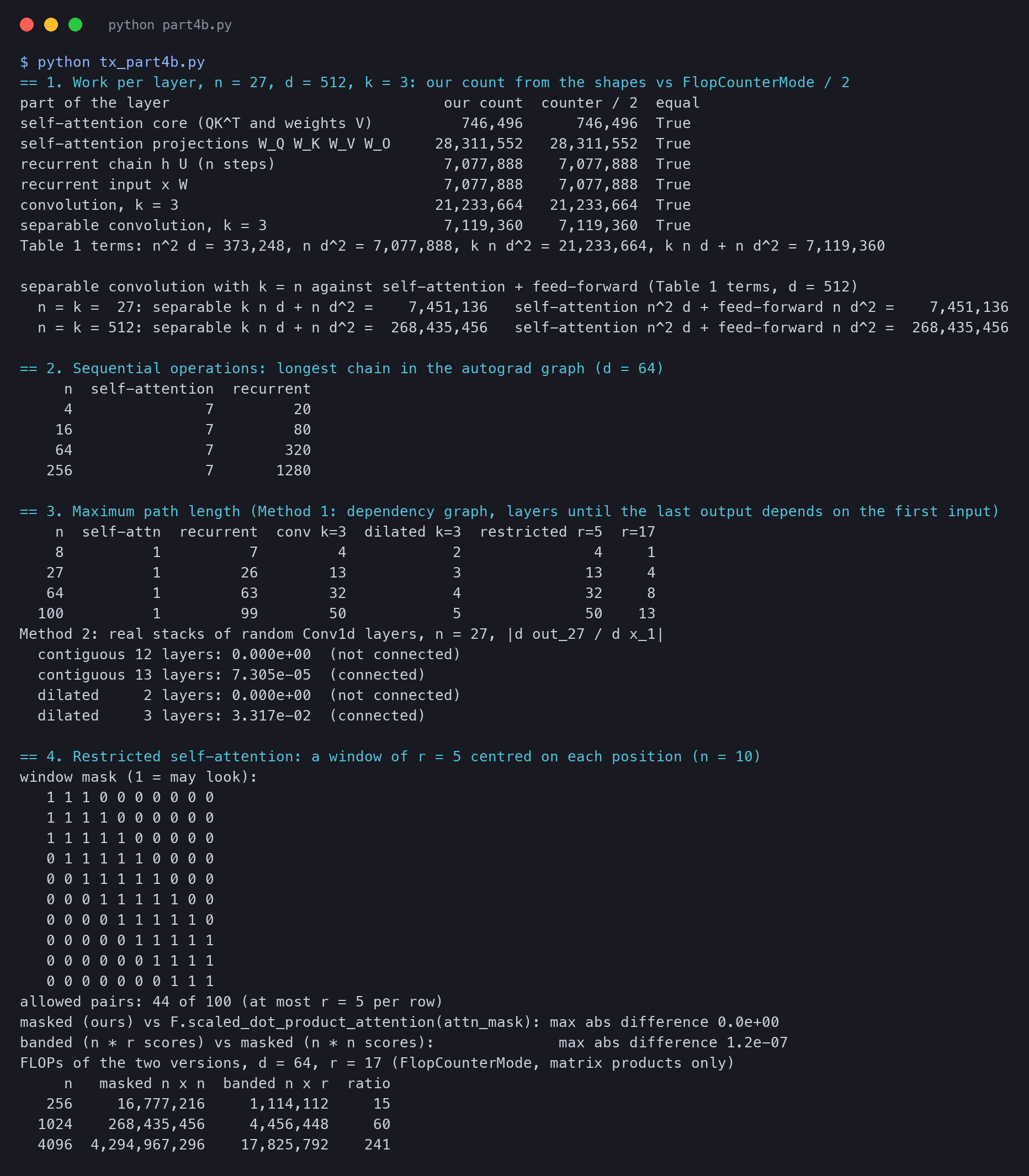
self-attention core (QK^T and weights V)          746,496      746,496  True
self-attention projections W_Q W_K W_V W_O     28,311,552   28,311,552  True
recurrent chain h U (n steps)                   7,077,888    7,077,888  True
recurrent input x W                             7,077,888    7,077,888  True
convolution, k = 3                             21,233,664   21,233,664  True
separable convolution, k = 3                    7,119,360    7,119,360  True
Table 1 terms: n^2 d = 373,248, n d^2 = 7,077,888, k n d^2 = 21,233,664, k n d + n d^2 = 7,119,360

Every row agrees to the last digit. So the formulas of Table 1 are not estimates. They are exact counts of the matrix products, without the constant factors. One of those factors is worth seeing. The attention core costs $2 n^2 d = 746{,}496$ , not $n^2 d = 373{,}248$ , because it has two products of that size: the scores and the mix. Big-O notation drops the 2.

The second lesson is the honest note above, now in numbers. The four projections of attention cost 28,311,552 multiply-adds, the attention core only 746,496. For a short sentence, the projections are most of the cost of a real attention layer, and the $n^2$ term is small. Table 1 leaves them out, because a recurrent layer has the same kind of term. It is the input product $x W$ , the row with 7,077,888.

From the paper§4

What it says

"a self-attention layer connects all positions with a constant number of sequentially executed operations, whereas a recurrent layer requires $O(n)$ sequential operations." Also, "self-attention layers are faster than recurrent layers when the sequence"...

What it means

Picture a relay race and a swimming race. In a relay, runner 2 cannot start before runner 1 hands over the baton. Four runners take four legs of time. In a swimming race, all swimmers start at the same moment. Eight swimmers take the time of one length.

A recurrent layer is a relay: the memory after word $t$ needs the memory after word $t-1$ . Self-attention is the swimming race. The scores of all $n \times n$ pairs are independent, so one large matrix product computes them all at once. That is why "sequential operations" is $O(n)$ for one and $O(1)$ for the other.

Counting the waiting steps in code

We can measure this column too. PyTorch records every operation of a computation in a graph, to compute the gradients later. Each operation points to the operations whose results it used. The longest chain in that graph is the number of steps that must run one after another, whatever the hardware.

python

def graph_depth(t):
    """The longest chain of operations from the output back to the inputs, in PyTorch's autograd graph.
    Operations on one chain must run one after another; operations on different chains can run in parallel."""
    memo = {}

    def depth(node):
        if node is None:
            return 0
        if node not in memo:
            parents = [p for p, _ in node.next_functions]
            memo[node] = 1 + max([depth(p) for p in parents] or [0])
        return memo[node]
    return depth(t.grad_fn)

def self_attention_layer(x, Wq, Wk, Wv):
    """A whole self-attention layer (one head): the projections, then the core."""
    return attention_core(x @ Wq, x @ Wk, x @ Wv)                            # (n, d)

def recurrent_layer(x, W, U):
    """A whole recurrent layer: the input part x W for all positions at once, then the chain."""
    return recurrent_chain(x @ W, U)

We give the weights requires_grad=True, so that PyTorch records the graph. Then we measure both layers for four lengths:

python

dd = 64
Aq, Ak, Av, Wr, Ur = (torch.randn(dd, dd, requires_grad=True) for _ in range(5))
for n2 in [4, 16, 64, 256]:
    xs = torch.randn(n2, dd)
    da = graph_depth(self_attention_layer(xs, Aq, Ak, Av))
    dr = graph_depth(recurrent_layer(xs, Wr, Ur))

plain text

== 2. Sequential operations: longest chain in the autograd graph (d = 64)
     n  self-attention  recurrent
     4               7         20
    16               7         80
    64               7        320
   256               7       1280

For self-attention, the longest chain has 7 operations at every length: a few matrix products, the scale and the softmax. A longer sentence makes each product larger, but it does not add a link to the chain. The recurrent chain grows in step with $n$ : 20 operations for 4 tokens, 1,280 for 256 tokens. This is the second column of Table 1, measured: $O(1)$ against $O(n)$ . A GPU can run the many multiplications inside one attention product at the same time. It cannot start step 2 of the recurrent chain before step 1 ends.

From the paper§4

What it says

Self-attention is faster "when the sequence length n is smaller than the representation dimensionality d, which is most often the case with sentence representations used by state-of-the-art models in machine translations, such as word-piece [38] and byte-pair [31] representations."

What it means

This is the $n / d$ ratio in words. The claim depends on one fact about the data: real sentences are short compared to 512. Word-piece and byte-pair are two ways to cut text into tokens. Common words stay whole, and rare words break into pieces. So the number of tokens is a little larger than the number of words, but not by much.

We can check the claim. The translation model that we use in this series, Helsinki-NLP/opus-mt-en-de, has $d = 512$ like the base Transformer. Its tokenizer is a close relative of byte-pair encoding. We gave it six English sentences, from 5 to 32 words long.

The tokenizer gives these lengths:

plain text

2. Real sentence lengths (Marian en-de tokenizer, d_model = 512)
  n =   8  words =  6  n/d = 0.016  The cat sat on the mat.
  n =   7  words =  5  n/d = 0.014  Attention is all you need.
  n =  13  words = 12  n/d = 0.025  The agreement on the European Economic Area was signed in Au...
  n =  23  words = 17  n/d = 0.045  Self-attention layers are faster than recurrent layers when ...
  n =  33  words = 26  n/d = 0.064  Learning long-range dependencies is a key challenge in many ...
  n =  39  words = 32  n/d = 0.076  The Transformer allows for significantly more parallelizatio...
  tokens of sentence 4: ▁Self - at tention ▁layers ▁are ▁faster ▁than ▁recurrent ▁layers ▁when ▁the ▁sequence ▁length ▁is ▁smaller ▁than ▁the ▁representation ▁dimension ality . </s>

Even the longest sentence, at 39 tokens, has $n / d = 0.076$ . So for this sentence the attention core does about 13 times less work than a recurrent layer of the same width. Each count includes the end-of-sentence token </s>. These six sentences are our own choice, not the paper's test set. They show the order of size, not an average over a corpus.

Time on a real computer

Counting multiplications is one thing. Does a real computer agree? Our script times one self-attention step against one recurrent loop, both with $d = 512$ . The attention step includes the three projections to queries, keys and values. The recurrent loop does its input projection for all words at once, then runs the chain of $n$ updates.

plain text

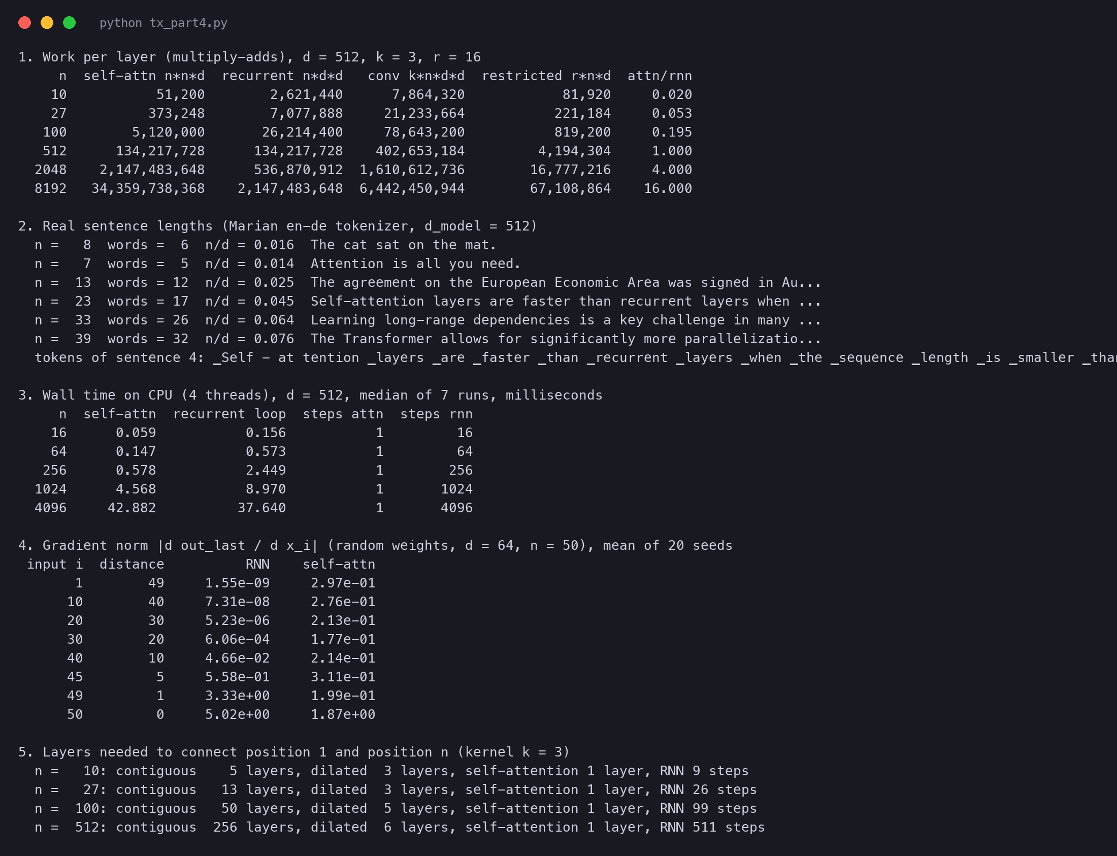
3. Wall time on CPU (4 threads), d = 512, median of 7 runs, milliseconds
     n  self-attn  recurrent loop  steps attn  steps rnn
    16      0.059           0.156           1         16
    64      0.147           0.573           1         64
   256      0.578           2.449           1        256
  1024      4.568           8.970           1       1024
  4096     42.882          37.640           1       4096

At 16 tokens, attention takes 0.059 ms and the loop takes 0.156 ms. At 1,024 tokens, attention is still about two times faster. At 4,096 tokens, the $n^2$ term wins and attention becomes the slower one, as the arithmetic predicts.

Two limits apply to this test. It ran on a laptop CPU with 4 threads, in PyTorch, with random weights and one batch of one sentence. A GPU runs the large matrix products of attention much faster, but cannot speed up the 4,096 small waiting steps of the loop. So we expect the gap at short lengths to be larger on a GPU, not smaller. We did not measure a GPU here.

The path between two words

From the paper§4

What it says

"Learning long-range dependencies is a key challenge in many sequence transduction tasks." One key factor is "the length of the paths forward and backward signals have to traverse in the network".

What it means

A long-range dependency is a link between two words far apart, like "keys ... are" above. The network must carry information along a path from one word to the other. The forward signal is the information itself, on its way to the output. The backward signal is the gradient, on its way back from the loss to the weights that must change.

Both signals pass through every step of the path, and each step can weaken or blur them. So the paper measures a layer by the longest path it creates between two positions. It does not count the work along the path, only the number of steps.

The third column of Table 1 is about learning, not speed. The figure below draws the three layers for a sentence of 8 words. The bold lines show the shortest route from word 1 to the output at word 8.

The maximum path length of Table 1, drawn for 8 words. A recurrent layer passes word 1 through a chain of 7 memory updates. A dilated convolution with kernel 3 reaches it in 2 layers. Self-attention reaches it in 1 step.

Why does a long path hurt? During training, the network learns from the gradient: a signal that says how much each input should change. In a recurrent layer, the gradient from word 8 to word 1 passes through 7 updates. Each update multiplies it by a matrix and by the slope of the tanh function. If these factors are a little smaller than 1, the product shrinks fast, like $0.6^7 \approx 0.03$ .

We measured this. Our script builds a recurrent network with tanh and a single self-attention layer, both with random weights. Each has vectors of 64 numbers and reads 50 positions. We compute the size of the gradient of the last output with respect to each input, and take the mean of 20 random networks.

plain text

4. Gradient norm |d out_last / d x_i| (random weights, d = 64, n = 50), mean of 20 seeds
 input i  distance          RNN    self-attn
       1        49     1.55e-09     2.97e-01
      10        40     7.31e-08     2.76e-01
      20        30     5.23e-06     2.13e-01
      30        20     6.06e-04     1.77e-01
      40        10     4.66e-02     2.14e-01
      45         5     5.58e-01     3.11e-01
      49         1     3.33e+00     1.99e-01
      50         0     5.02e+00     1.87e+00

How strongly the last output depends on each input, against the distance between them (log scale). In the recurrent network the gradient falls by about 10 to the power 9 over 49 positions. In one self-attention layer it stays between about 0.18 and 0.31 at every distance above 0. Random weights, 64 numbers per vector, mean of 20 networks.

The numbers tell the story of the third column. In the recurrent network, the first word has a gradient of $1.55 \times 10^{-9}$ , about three billion times smaller than the last word. In practice, such a word cannot teach the network anything. In the attention layer, the first word gets 0.297 and the 49th word gets 0.199. Distance does not matter.

This test has limits too. The weights are random, not trained. A trained LSTM keeps gradients much better than our plain tanh network, because its gates were designed for this problem. And the input at distance 0 is larger in attention because it also feeds the query of the last position. The test shows the shape of the effect, not the size it has in a real trained model.

The path length in code

The figure above draws the paths for 8 words. Code can count them for any length. The idea is to describe one layer by a table of links. Entry $(i, j)$ is True if output $i$ reads input $j$ directly. A stack of layers is the product of their tables, with True and False in place of numbers. We stack layers until the last output depends on the first input.

python

def window_links(n, offsets):
    """links[i, j] = True if output i of one layer reads input j directly, for j = i + offset.
    A one-sided kernel of width 3 has offsets (0, -1, -2); dilated by 3 it has (0, -3, -6)."""
    links = torch.zeros(n, n, dtype=torch.bool)
    for i in range(n):
        for o in offsets:
            if 0 <= i + o < n:
                links[i, i + o] = True
    return links

def layers_to_connect(n, layer_links):
    """Stack layers until the last output depends on the first input; return how many layers that takes.
    layer_links(L) gives the links of layer L. The dependency of a stack is the boolean product of its layers."""
    reach = torch.eye(n, dtype=torch.bool)           # before any layer, each position depends only on itself
    for L in range(1, 10 * n):
        reach = (layer_links(L).int() @ reach.int()) > 0
        if reach[n - 1, 0]:                          # output n now depends on input 1
            return L
    return None

def recurrent_path(n):
    """x_1 enters the memory at h_1. To reach the output z_n = h_n, it must pass h_1 -> h_2 -> ... -> h_n."""
    t, hops = 1, 0                        # x_1 is now inside h_1
    while t < n:
        t += 1                            # one recurrent step: h_t is computed from h_(t-1)
        hops += 1
    return hops

Each layer type is one table of links. Self-attention links every pair. A convolution with kernel 3 links each output to its own position and the two before it. A dilated convolution spreads the same three links further apart in each layer: 1, 3 and 9 positions. Restricted attention links each output to the $r$ inputs centred on it.

python

k = 3
for n2 in [8, 27, 64, 100]:
    full = torch.ones(n2, n2, dtype=torch.bool)
    p_attn = layers_to_connect(n2, lambda L: full)                                       # every query sees every key
    p_conv = layers_to_connect(n2, lambda L: window_links(n2, [0, -1, -2]))               # kernel 3, contiguous
    p_dil = layers_to_connect(n2, lambda L: window_links(n2, [0, -k ** (L - 1), -2 * k ** (L - 1)]))   # dilation 1, 3, 9, ...
    p_loc = layers_to_connect(n2, lambda L: window_links(n2, range(-2, 3)))               # window of r = 5, centred
    p_loc17 = layers_to_connect(n2, lambda L: window_links(n2, range(-8, 9)))             # window of r = 17, centred
    p_rnn = recurrent_path(n2)

plain text

    n  self-attn  recurrent  conv k=3  dilated k=3  restricted r=5  r=17
    8          1          7         4            2               4     1
   27          1         26        13            3              13     4
   64          1         63        32            4              32     8
  100          1         99        50            5              50    13

Read the row for $n = 27$ . Self-attention needs 1 layer, the recurrent layer 26 steps, the contiguous convolution 13 layers and the dilated convolution 3. These are the counts of Table 1: $O(1)$ , $O(n)$ , $O(n/k)$ and $O(\log_k n)$ . The last two columns are restricted attention. With a window of 5, it needs 13 layers, because each layer reaches only 2 positions further. A window of 17 reaches 8 positions per layer and needs 4: the $O(n/r)$ of the last row of Table 1.

Our convolutions are one-sided: each output looks only at its own position and earlier ones. The decoder of ByteNet, reference [18] of the paper, works this way. Their reach matches the $\log_k(n)$ of the paper exactly. A centred kernel reaches as many positions, but half of them on each side.

When sentences get long

From the paper§4

What it says

"To improve computational performance for tasks involving very long sequences, self-attention could be restricted to considering only a neighborhood of size r ... This would increase the maximum path length to $O(n/r)$ . We plan to investigate this approach further in future work."

What it means

The authors saw the weak point in their own table. The $n^2$ term is harmless for sentences but grows fast for whole documents. Their fix is a window. Each word looks only at the $r$ words around it, so the cost falls from $n^2 \cdot d$ to $r \cdot n \cdot d$ .

The price is the path. Word 1 can no longer see word 1,000 in one step. The signal must hop from window to window, about $n / r$ hops. With $n = 8{,}192$ and $r = 16$ , the core cost falls from about 34 billion to about 67 million multiplications, 512 times less. But the longest path grows from 1 to about 512 hops.

"Future work" turned out to be a large field. Many later models for long text use some form of local or sparse attention, often with a few global tokens to keep paths short. The trade-off in this one sentence is the same trade-off they all balance.

Restricted attention in code

The window is one more mask, like the decoder mask of Part 3. Query $i$ may look at key $j$ only if the two are at most $\lfloor r/2 \rfloor$ positions apart. Here is the mask for 10 tokens and a window of $r = 5$ , built with two loops:

python

n2, r = 10, 5
half = r // 2
local = torch.zeros(n2, n2, dtype=torch.bool)
for i in range(n2):
    for j in range(n2):
        local[i, j] = abs(i - j) <= half        # key j is inside the window of query i

plain text

window mask (1 = may look):
   1 1 1 0 0 0 0 0 0 0
   1 1 1 1 0 0 0 0 0 0
   1 1 1 1 1 0 0 0 0 0
   0 1 1 1 1 1 0 0 0 0
   0 0 1 1 1 1 1 0 0 0
   0 0 0 1 1 1 1 1 0 0
   0 0 0 0 1 1 1 1 1 0
   0 0 0 0 0 1 1 1 1 1
   0 0 0 0 0 0 1 1 1 1
   0 0 0 0 0 0 0 1 1 1
allowed pairs: 44 of 100 (at most r = 5 per row)

The mask is a band along the diagonal. Each row has at most 5 ones. The rows at the two ends have fewer, because their window runs past the end of the sentence. Our attention function with this mask gives the same output as the library with the same mask.

python

def masked_attention(q, k, v, mask):
    """Equation 1 with a mask: computes all n x n scores, then hides the ones outside the window."""
    scores = q @ k.T / math.sqrt(q.shape[-1])
    scores = scores.masked_fill(~mask, float('-inf'))
    return torch.softmax(scores, dim=-1) @ v

There is a catch. The masked version still computes all $n \times n$ scores, and then throws most of them away. It saves no work at all. To get the $r \cdot n \cdot d$ of Table 1, the code must compute only the scores inside the window. banded_attention does that. For each query, it cuts out the $r$ keys and values of its window with unfold, and computes $r$ dot products.

python

def banded_attention(q, k, v, r):
    """The same result, but each query computes only its r scores: n * r work in place of n * n."""
    n, d = q.shape
    half = r // 2
    kp = F.pad(k, (0, 0, half, half))                # (n + 2 half, d): zero rows before the start and after the end
    vp = F.pad(v, (0, 0, half, half))
    k_win = kp.unfold(0, r, 1)                       # (n, d, r): for query i, the keys i - half ... i + half
    v_win = vp.unfold(0, r, 1)                       # (n, d, r)
    scores = (q.unsqueeze(1) @ k_win).squeeze(1) / math.sqrt(d)    # (n, r): r dot products per query
    pos = torch.arange(n).unsqueeze(1) + torch.arange(r) - half      # (n, r): the real position of each window slot
    scores = scores.masked_fill((pos < 0) | (pos >= n), float('-inf'))   # slots outside the sentence are padding
    w = torch.softmax(scores, dim=-1)                # (n, r)
    return (v_win @ w.unsqueeze(2)).squeeze(2)       # (n, d): mix the r values of each window

q, kk, v = torch.randn(n2, 16), torch.randn(n2, 16), torch.randn(n2, 16)
o_mask = masked_attention(q, kk, v, local)
o_lib = F.scaled_dot_product_attention(q, kk, v, attn_mask=local)
o_band = banded_attention(q, kk, v, r)
d_lib = (o_mask - o_lib).abs().max().item()       # Method 1 (our mask) against Method 2 (the library)
d_band = (o_band - o_mask).abs().max().item()     # the banded version against the masked one

plain text

masked (ours) vs F.scaled_dot_product_attention(attn_mask): max abs difference 0.0e+00
banded (n * r scores) vs masked (n * n scores):              max abs difference 1.2e-07

Restricted self-attention for 10 tokens and a window of 5. Left: the mask, a band of 44 allowed pairs in a table of 100. Right: the same band stored as 10 rows of 5 slots, so that only the scores inside the window are computed. The number in each slot is the position of its key; empty slots at the two ends are padding.

The banded version matches the masked one to $1.2 \times 10^{-7}$ , and the masked one matches the library exactly. Now count the work. We ran both versions under the FLOP counter, with $d = 64$ and a window of 17:

python

d3, r3 = 64, 17
for n3 in [256, 1024, 4096]:
    q, kk, v = torch.randn(n3, d3), torch.randn(n3, d3), torch.randn(n3, d3)
    mask = (torch.arange(n3).unsqueeze(1) - torch.arange(n3)).abs() <= r3 // 2
    fm = flops(masked_attention, q, kk, v, mask)
    fb = flops(banded_attention, q, kk, v, r3)               # window of 17: 8 on each side and the centre

plain text

FLOPs of the two versions, d = 64, r = 17 (FlopCounterMode, matrix products only)
     n   masked n x n  banded n x r  ratio
   256     16,777,216     1,114,112     15
  1024    268,435,456     4,456,448     60
  4096  4,294,967,296    17,825,792    241

At 256 tokens, the band does 15 times less work than the full table. At 4,096 tokens, it does 241 times less, and the gap keeps growing with $n$ . That is the gain the authors had in mind. The price is the path: the table of the previous section showed that a window of 17 needs 13 layers to connect 100 tokens.

Why not convolutions?

From the paper§4

What it says

"A single convolutional layer with kernel width k < n does not connect all pairs of input and output positions. Doing so requires a stack of $O(n/k)$ convolutional layers in the case of contiguous kernels, or $O(\log_k(n))$ in the case of dilated convolutions." They are "more expensive than recurrent layers, by a factor of k". Even a separable convolution with $k = n$ costs the same as "the combination of a self-attention layer and a point-wise feed-forward layer, the approach we take in our model."

What it means

A convolution is a small window that slides along the sentence. With kernel width $k = 3$ , each output sees one word on each side. To see further, you stack layers: two layers see 5 words, three layers see 7. Each layer adds $k - 1 = 2$ words of reach. A dilated convolution spreads its window out: layer 1 looks at neighbours, layer 2 at positions 3 apart, layer 3 at positions 9 apart. Then the reach grows as $k^L$ , much faster.

The cost is $k$ times the recurrent cost, because each output mixes $k$ input vectors with a $d \times d$ matrix each. ConvS2S and ByteNet, the models from Part 1 that used convolutions, paid this cost to get rid of the waiting steps of recurrence. Self-attention removes the waiting steps too, and also makes the path short.

The last two sentences, about separable convolutions, get their own box below, with a count in code.

Our script counts the layers that a kernel of width 3 needs to connect the first and the last word:

plain text

5. Layers needed to connect position 1 and position n (kernel k = 3)
  n =   10: contiguous    5 layers, dilated  3 layers, self-attention 1 layer, RNN 9 steps
  n =   27: contiguous   13 layers, dilated  3 layers, self-attention 1 layer, RNN 26 steps
  n =  100: contiguous   50 layers, dilated  5 layers, self-attention 1 layer, RNN 99 steps
  n =  512: contiguous  256 layers, dilated  6 layers, self-attention 1 layer, RNN 511 steps

The formulas behind the counts: $L$ contiguous layers reach $1 + L(k-1)$ positions, and $L$ dilated layers reach $k^L$ . For $n = 27$ , contiguous layers need $\lceil 26 / 2 \rceil = 13$ , and dilated layers need $\log_3 27 = 3$ , because $3^3 = 27$ . Self-attention needs 1 layer for every $n$ .

From the paper§4

What it says

Connecting all positions "requires a stack of $O(n/k)$ convolutional layers in the case of contiguous kernels, or $O(\log_k(n))$ in the case of dilated convolutions [18], increasing the length of the longest paths between any two positions in the network."

What it means

The key words are at the end: "increasing the length of the longest paths". A stack of convolutions does connect word 1 and word 27 in the end. But the connection runs through every layer of the stack, so the path is as long as the stack. Dilation makes the stack short, but its height still grows with $n$ .

Reference [18] is ByteNet, a translation model built from dilated convolutions. Its reach doubles or triples with each layer, which is why its path grows only as a logarithm of $n$ .

The tables of links in the path section are one method to count these layers. A second method uses real layers. We build a stack of random one-sided convolutions and ask autograd whether the last output depends on the first input at all. If the gradient is exactly 0, no path exists.

python

def conv_stack_grad(n, L, dilated=False):
    """Method 2: a real stack of L random one-sided Conv1d layers (kernel 3). Is d out_n / d x_1 zero?"""
    g = torch.Generator().manual_seed(L)
    x = torch.randn(1, 8, n, generator=g, requires_grad=True)         # 8 channels, n positions
    h = x
    for l in range(L):
        dil = 3 ** l if dilated else 1
        w = torch.randn(8, 8, 3, generator=g)
        h = F.pad(h, (2 * dil, 0))                                     # pad on the left only: output t reads t, t - dil, t - 2 dil
        h = torch.tanh(F.conv1d(h, w, dilation=dil))
    h[0, :, n - 1].sum().backward()                                    # the last output ...
    return x.grad[0, :, 0].abs().sum().item()                          # ... and its gradient at the first input

for L, dil in [(12, False), (13, False), (2, True), (3, True)]:
    gsum = conv_stack_grad(27, L, dil)

plain text

Method 2: real stacks of random Conv1d layers, n = 27, |d out_27 / d x_1|
  contiguous 12 layers: 0.000e+00  (not connected)
  contiguous 13 layers: 7.305e-05  (connected)
  dilated     2 layers: 0.000e+00  (not connected)
  dilated     3 layers: 3.317e-02  (connected)

With 12 contiguous layers, the gradient is exactly 0: no path exists from word 1 to the output at word 27. With 13 layers, a path appears. The dilated stack connects in 3 layers and not in 2. Both methods give the counts of the formulas above.

From the paper§4

What it says

"Separable convolutions [6], however, decrease the complexity considerably, to $O(k \cdot n \cdot d + n \cdot d^2)$ . Even with $k = n$ , however, the complexity of a separable convolution is equal to the combination of a self-attention layer and a point-wise feed-forward layer, the approach we take in our model."

What it means

This is a neat argument. A separable convolution splits the work into a cheap per-channel window and a $d \times d$ mix. With a window as wide as the whole sentence, its cost equals one attention layer plus one feed-forward layer. That pair is exactly one Transformer block from Part 2. So the Transformer reaches the full sentence for the price of the most efficient convolution.

Our count table above has a row for it. With $k = 3$ and 27 tokens, the separable convolution needs 7,119,360 multiply-adds, against 21,233,664 for the ordinary one. The FLOP counter agrees on both.

With $k = n$ , the term $k \cdot n \cdot d$ becomes $n^2 \cdot d$ , the cost of self-attention, and $n \cdot d^2$ is the cost of a point-wise feed-forward layer. The Transformer pays what the cheapest full-width convolution would pay, and gets a path of length 1.

A side benefit: we can look inside

From the paper§4

What it says

"As side benefit, self-attention could yield more interpretable models." The authors inspect attention distributions and find that "individual attention heads clearly learn to perform different tasks, many appear to exhibit behavior related to the syntactic and semantic structure of the sentences."

What it means

In a recurrent network, the memory is one vector of 512 numbers that mixes everything read so far. It is hard to say which earlier word caused what. In attention, each head writes down an explicit table: for this word, how much weight on each other word. We can print that table and read it.

The paper shows such tables in its appendix, with heads that link a pronoun to its noun, and Part 6 looks at them. Be careful with the word "could". An attention weight shows where a head looked, not always why the model gave its answer. Later research found that attention maps are a useful clue, but not a full explanation.

The three wishes, scored

Put the three measures side by side for a typical sentence of 27 tokens and $d = 512$ :

layer	work of the core	waiting steps	longest path
self-attention	373,248	1	1
recurrent	7,077,888	27	27
convolution, $k = 3$ , contiguous	21,233,664	1	13 layers
convolution, $k = 3$ , dilated	21,233,664	1	3 layers

For sentences, self-attention wins all three columns. That is the whole argument of Section 4. It does not say that attention is better for every input. For very long inputs, the $n^2$ cost returns, and the authors say so.

Key takeaways

Section 4 scores a layer on three measures: work per layer, steps that must wait for each other, and the longest path between two positions.
Self-attention costs $O(n^2 \cdot d)$ and a recurrent layer costs $O(n \cdot d^2)$ . Their ratio is $n / d$ .
With $d = 512$ , self-attention does less core work whenever a sentence has fewer than 512 tokens. Our six test sentences had 7 to 39 tokens.
Self-attention has one sequential step; a recurrent layer has $n$ . On our CPU, attention was faster up to 1,024 tokens and slower at 4,096.
Any word reaches any other word in one attention step. In our random networks, the recurrent gradient fell to $1.55 \times 10^{-9}$ over 49 positions; the attention gradient stayed near 0.2.
Convolutions need a stack of layers to connect distant words: 13 contiguous or 3 dilated layers for 27 tokens with $k = 3$ .
Restricted attention with a window $r$ cuts the cost to $O(r \cdot n \cdot d)$ but makes the path $O(n / r)$ .
Table 1 counts only the parts that grow differently. The projections add about $4 \cdot n \cdot d^2$ to a real attention layer.
Counted from the shapes in code, every layer matched PyTorch's FLOP counter exactly. For 27 tokens, the attention core is 746,496 multiply-adds and its four projections 28,311,552.
The longest chain in the autograd graph stayed at 7 operations for self-attention and grew to 1,280 for a recurrent layer of 256 tokens.
A mask alone does not make restricted attention cheap. A banded version that computes only the window did 241 times less work at 4,096 tokens.

The paper and the code

Paper (arXiv 1706.03762) · Official code (tensor2tensor) · Our scripts for this series

Why Self-Attention: Cost, Steps and Paths

Three measures for a layer#

Table 1, cell by cell#

The first column: work per layer#

Counting the work in code#

Counting the waiting steps in code#

Time on a real computer#

The path between two words#

The path length in code#

When sentences get long#

Restricted attention in code#

Why not convolutions?#

A side benefit: we can look inside#

The three wishes, scored#

The paper and the code#

Three measures for a layer

Table 1, cell by cell

The first column: work per layer

Counting the work in code

Counting the waiting steps in code

Time on a real computer

The path between two words

The path length in code

When sentences get long

Restricted attention in code

Why not convolutions?

A side benefit: we can look inside

The three wishes, scored

The paper and the code