Transformer, explained · Part 3 of 7 · Covers §3.2, Figure 2, Equation 1, footnote 4, §3.2.2, §3.2.3

Attention: Queries, Keys and Values

How one attention step works, why the scores are divided by the square root of the key size, and why the model runs eight heads side by side. We write attention and multi-head attention from scratch in Python, match them with the PyTorch library and with a released translation model, and show three common bugs.

Attention Is All You Need. Ashish Vaswani, Noam Shazeer, Niki Parmar, Jakob Uszkoreit, Llion Jones, Aidan N. Gomez, Łukasz Kaiser, Illia Polosukhin. NeurIPS 2017, 2017. arXiv:1706.03762

Attention is the one step in the Transformer where a word gets information from other words. Each piece below shows the exact lines of the paper, then explains them, and then checks them on a real translation model.

What an attention function is#

Figure 2: the two pictures of attention#

Scaled dot-product attention#

Equation 1, step by step#

The equation does four things in order: score every pair, shrink the scores, turn them into weights, mix the values.

Read it from left to right:

• $Q$ is a table with one row for each query token. Each row has $d_k$ numbers.
• $K$ is a table with one row for each key token, also $d_k$ numbers per row. $K^\top$ is the same table turned on its side.
• $Q K^\top$ is the table of all dot products. Row $i$, column $j$ is the score of query $i$ against key $j$.
• $\sqrt{d_k}$ divides every score by the same number. The next section explains why.
• $\text{softmax}$ works on each row on its own. Each row becomes weights that add up to 1.
• $V$ is the table of values. The weights multiply $V$, so each output row is a weighted average of the value rows.

A tiny example with three tokens and $d_k = 2$. The three queries are $(1, 0)$, $(0, 1)$ and $(1, 1)$. The three keys are $(2, 0)$, $(0, 2)$ and $(1, 1)$. The three values are $(10, 0)$, $(0, 10)$ and $(5, 5)$.

Take the first query, $(1, 0)$. Its dot products with the three keys are 2, 0 and 1. Divide by $\sqrt{2} = 1.414$, and the scores are 1.414, 0 and 0.707. The softmax gives:

The output is $0.576 \times (10, 0) + 0.140 \times (0, 10) + 0.284 \times (5, 5) = (7.18, 2.82)$. The query points along the first axis, like the first key, so the output is mostly the first value. Our script gives the same numbers:

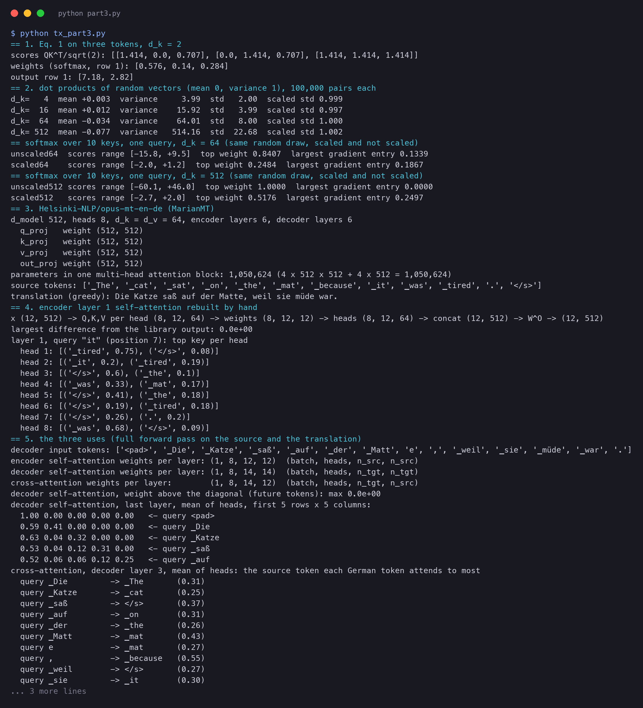
== 1. Eq. 1 on three tokens, d_k = 2
scores QK^T/sqrt(2): [[1.414, 0.0, 0.707], [0.0, 1.414, 0.707], [1.414, 1.414, 1.414]]
weights (softmax, row 1): [0.576, 0.14, 0.284]
output row 1: [7.18, 2.82]

Look at the third row of scores: 1.414 three times. The query $(1, 1)$ matches all three keys equally, so it gets one third of each value. Attention can share its focus when nothing stands out.

Method 1: Equation 1 from scratch, every matrix printed#

Here is the same computation as code, so you can follow each table. NumPy is a Python library for tables of numbers. In NumPy, @ is the matrix product and .T turns a table on its side.

Q = np.array([[1., 0.], [0., 1.], [1., 1.]])     # 3 queries, one row per token
K = np.array([[2., 0.], [0., 2.], [1., 1.]])     # 3 keys
V = np.array([[10., 0.], [0., 10.], [5., 5.]])   # 3 values
d_k = Q.shape[1]                                  # 2 numbers per query and key

scores = Q @ K.T                                  # (3, 3): row i, column j = query i . key j
scaled = scores / np.sqrt(d_k)                    # divide every score by sqrt(2) = 1.414
e = np.exp(scaled - scaled.max(axis=1, keepdims=True))  # subtract the row maximum first: same softmax, no overflow
weights = e / e.sum(axis=1, keepdims=True)        # each row now adds up to 1
out = weights @ V                                 # (3, 2): each output row is a weighted average of the value rows

The script prints every table on the way:

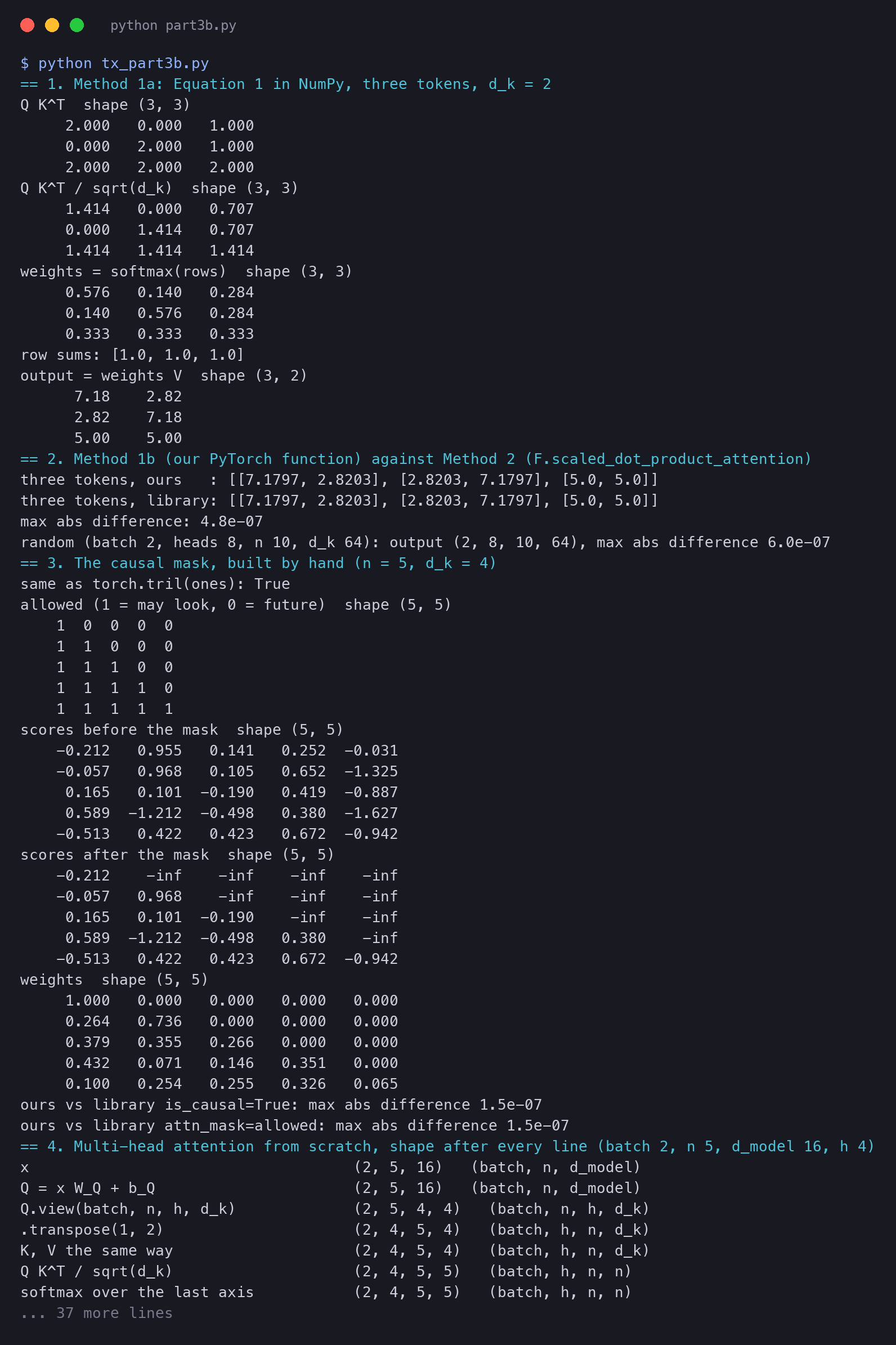
Q K^T  shape (3, 3)
     2.000   0.000   1.000
     0.000   2.000   1.000
     2.000   2.000   2.000
Q K^T / sqrt(d_k)  shape (3, 3)
     1.414   0.000   0.707
     0.000   1.414   0.707
     1.414   1.414   1.414
weights = softmax(rows)  shape (3, 3)
     0.576   0.140   0.284
     0.140   0.576   0.284
     0.333   0.333   0.333
row sums: [1.0, 1.0, 1.0]
output = weights V  shape (3, 2)
      7.18    2.82
      2.82    7.18
      5.00    5.00

Read the tables in order. Q K^T holds the raw dot products: row 1 is 2, 0 and 1, as we computed by hand. The next table is the same divided by 1.414. The softmax turns each row into weights, and the row sums show that each row adds up to 1. The last table is the output, and its row 1 is (7.18, 2.82), as above.

One line needs a word. Before the exponential, the code subtracts the largest score of each row. This does not change the softmax, because the same factor $e^{-m}$ appears above and below the fraction. It only keeps $e^{s}$ from growing too large for the computer when a score is big.

Method 2: the library function#

PyTorch is the library that most Transformer code uses today. Below is Equation 1 as a PyTorch function, which the rest of this page uses again and again. It also takes an optional mask, which the section on the decoder mask explains. The lines of the body follow the boxes of Figure 2: MatMul and Scale, then Mask, SoftMax and the last MatMul.

def attention(Q, K, V, mask=None):
    """Equation 1: softmax(Q K^T / sqrt(d_k)) V.
    Q: (..., n_q, d_k)   K: (..., n_k, d_k)   V: (..., n_k, d_v)
    mask: True where a query may look at a key, False where it may not (None = no mask)."""
    d_k = Q.shape[-1]
    scores = Q @ K.transpose(-2, -1) / math.sqrt(d_k)       # (..., n_q, n_k): every query against every key
    if mask is not None:
        scores = scores.masked_fill(~mask, float('-inf'))    # forbidden pairs get minus infinity, BEFORE the softmax
    weights = torch.softmax(scores, dim=-1)                  # (..., n_q, n_k): each row adds up to 1
    return weights @ V, weights                              # (..., n_q, d_v), (..., n_q, n_k)

PyTorch also has its own version, torch.nn.functional.scaled_dot_product_attention. We call both on the three tokens, and then on random tensors with the shape of a real attention step:

Qt, Kt, Vt = (torch.tensor(a, dtype=torch.float32) for a in (Q, K, V))
ours, _ = attention(Qt, Kt, Vt)                       # Method 1: our function
lib = F.scaled_dot_product_attention(Qt, Kt, Vt)       # Method 2: the library
d1 = (ours - lib).abs().max().item()                   # the largest difference over all outputs
q, k, v = torch.randn(2, 8, 10, 64), torch.randn(2, 8, 10, 64), torch.randn(2, 8, 10, 64)   # (batch, heads, n, d_k)
ours, _ = attention(q, k, v)
lib = F.scaled_dot_product_attention(q, k, v)
d2 = (ours - lib).abs().max().item()

three tokens, ours   : [[7.1797, 2.8203], [2.8203, 7.1797], [5.0, 5.0]]
three tokens, library: [[7.1797, 2.8203], [2.8203, 7.1797], [5.0, 5.0]]
max abs difference: 4.8e-07
random (batch 2, heads 8, n 10, d_k 64): output (2, 8, 10, 64), max abs difference 6.0e-07

The two methods agree to within $6 \times 10^{-7}$. That is not an error in either one. A computer stores each number of this kind with about 7 correct digits, and the library can add the products in a different order. The second test has 2 sentences, 8 heads, 10 tokens and 64 numbers per head. The @ product works on the last two axes and repeats for every sentence and head, so one function handles both cases.

Dot product or additive attention#

Why divide by the square root of d_k#

The equation behind the footnote, with its assumption:

Read it: the variance of the dot product is the sum of the variances of its $d_k$ terms. This holds when the terms are independent. Each term has variance 1 when $q_i$ and $k_i$ have mean 0 and variance 1. Dividing a random number by $c$ divides its variance by $c^2$, so dividing by $\sqrt{d_k}$ divides the variance by $d_k$.

A tiny check by hand with $d_k = 4$: each term is about $\pm 1$, so a sum of four terms often lands near $\pm 2$, which is $\sqrt{4}$. Our script drew 100,000 random pairs for four sizes:

== 2. dot products of random vectors (mean 0, variance 1), 100,000 pairs each
d_k=   4  mean +0.003  variance     3.99  std   2.00  scaled std 0.999
d_k=  16  mean +0.012  variance    15.92  std   3.99  scaled std 0.997
d_k=  64  mean -0.034  variance    64.01  std   8.00  scaled std 1.000
d_k= 512  mean -0.077  variance   514.16  std  22.68  scaled std 1.002

The variance follows $d_k$, as the footnote says, and the scaled std stays at 1.00. Next, what this does to the softmax. We took one random query and ten random keys, and computed the weights with and without the scale. We also computed the largest entry of the softmax gradient (its Jacobian matrix). For a softmax, no entry can be larger than 0.25.

== softmax over 10 keys, one query, d_k = 64 (same random draw, scaled and not scaled)
unscaled64  scores range [-15.8, +9.5]  top weight 0.8407  largest gradient entry 0.1339
scaled64    scores range [-2.0, +1.2]  top weight 0.2484  largest gradient entry 0.1867
== softmax over 10 keys, one query, d_k = 512 (same random draw, scaled and not scaled)
unscaled512 scores range [-60.1, +46.0]  top weight 1.0000  largest gradient entry 0.0000
scaled512   scores range [-2.7, +2.0]  top weight 0.5176  largest gradient entry 0.2497

With $d_k = 512$ and no scale, the scores spread from $-60$ to $+46$. The softmax puts a weight of 1.0000 on one key, and every gradient entry rounds to 0.0000. That attention head cannot learn. With the scale, the same vectors give a top weight of 0.52 and a gradient entry of 0.25, the largest a softmax allows. This is a toy with random vectors, not a trained model, but it shows the effect the paper describes.

Multi-head attention#

The multi-head equation#

Read it from the right. $W_i^Q$, $W_i^K$ and $W_i^V$ are the three matrices of head $i$, each of size $512 \times 64$. They turn the inputs into the queries, keys and values of that head. $\text{Attention}$ is Equation 1. $\text{Concat}$ puts the $h$ outputs side by side. $W^O$, of size $512 \times 512$, mixes them.

The parameter count with the base shapes: each head has three matrices of $512 \times 64$, and eight heads give $3 \times 8 \times 512 \times 64 = 786{,}432$ numbers. That is exactly three matrices of $512 \times 512$. Add $W^O$ and one bias vector of 512 for each of the four matrices:

Multi-head attention from scratch, line by line#

The multi-head equation hides one trick of the code. The paper writes $h$ separate matrices $W_i^Q$. Code keeps them side by side as one wide matrix $W^Q$ of size $d_{\text{model}} \times d_{\text{model}}$. It makes the queries of all heads with one product, and then cuts the result into $h$ pieces. The cut is two calls: view and transpose.

We follow a small example with real tensors: 2 sentences of 5 tokens, $d_{\text{model}} = 16$ and $h = 4$ heads, so $d_k = 4$. The comment at the end of a line says what it does.

batch, n, d_model, h = 2, 5, 16, 4
d_k = d_model // h                                  # 4 numbers per head
x = torch.randn(batch, n, d_model)                  # the input: 2 sentences of 5 tokens, 16 numbers each
p = {f'W_{m}': torch.randn(d_model, d_model) / math.sqrt(d_model) for m in 'QKVO'}   # paper layout: x @ W
p.update({f'b_{m}': torch.randn(d_model) * 0.1 for m in 'QKVO'})

Qm = x @ p['W_Q'] + p['b_Q']                         # all 4 heads' queries in one product
Qs = Qm.view(batch, n, h, d_k)                       # cut the last axis into h pieces of d_k
Qh = Qs.transpose(1, 2)                              # move heads before tokens: each head is its own problem
Kh = (x @ p['W_K'] + p['b_K']).view(batch, n, h, d_k).transpose(1, 2)   # keys: the same three steps
Vh = (x @ p['W_V'] + p['b_V']).view(batch, n, h, d_k).transpose(1, 2)   # values: the same three steps
S = Qh @ Kh.transpose(-2, -1) / math.sqrt(d_k)       # one n x n score table per head
Wt = torch.softmax(S, dim=-1)                        # each row of each table adds up to 1
heads = Wt @ Vh                                      # each head mixes its own values
merged = heads.transpose(1, 2)                       # tokens first again
concat = merged.reshape(batch, n, h * d_k)           # the h pieces side by side: the paper's Concat
y_steps = concat @ p['W_O'] + p['b_O']               # W^O mixes what the heads found

The script prints the shape after every line:

x                                    (2, 5, 16)   (batch, n, d_model)
Q = x W_Q + b_Q                      (2, 5, 16)   (batch, n, d_model)
Q.view(batch, n, h, d_k)             (2, 5, 4, 4)   (batch, n, h, d_k)
.transpose(1, 2)                     (2, 4, 5, 4)   (batch, h, n, d_k)
K, V the same way                    (2, 4, 5, 4)   (batch, h, n, d_k)
Q K^T / sqrt(d_k)                    (2, 4, 5, 5)   (batch, h, n, n)
softmax over the last axis           (2, 4, 5, 5)   (batch, h, n, n)
weights V                            (2, 4, 5, 4)   (batch, h, n, d_k)
.transpose(1, 2)                     (2, 5, 4, 4)   (batch, n, h, d_k)
.reshape(batch, n, h * d_k)          (2, 5, 16)   (batch, n, d_model)
concat W_O + b_O                     (2, 5, 16)   (batch, n, d_model)

Three lines do the real work. view(batch, n, h, d_k) reads the 16 numbers of each token as 4 groups of 4. No number moves; only the way we count them changes. transpose(1, 2) swaps the token axis and the head axis. Now the tensor is a stack of $2 \times 4 = 8$ small problems, one for each sentence and head.

Equation 1 then runs on all 8 problems at once, because @ repeats over the leading axes. The scores have the shape (2, 4, 5, 5): one 5 × 5 table for each sentence and head. The way back is the mirror image. transpose(1, 2) puts the tokens first again, and reshape glues the 4 pieces of each token into 16 numbers. That is the paper's Concat, and $W^O$ then mixes the pieces.

The block as three functions#

The same steps fit in three short functions. split_heads and merge_heads are the two reshapes. multi_head_attention is the multi-head equation. It takes two inputs: x_q makes the queries, and x_kv makes the keys and values. For self-attention we pass the same tensor twice; for cross-attention we pass two different ones.

def split_heads(t, h):
    """(batch, n, d_model) -> (batch, h, n, d_k): cut each token vector into h pieces, one per head."""
    batch, n, d_model = t.shape
    return t.view(batch, n, h, d_model // h).transpose(1, 2)

def merge_heads(t):
    """(batch, h, n, d_k) -> (batch, n, h * d_k): put the h pieces of each token side by side (Concat)."""
    batch, h, n, d_k = t.shape
    return t.transpose(1, 2).reshape(batch, n, h * d_k)

def multi_head_attention(x_q, x_kv, p, h, mask=None):
    """MultiHead(Q, K, V) = Concat(head_1, ..., head_h) W^O, with head_i = Attention(Q W_i^Q, K W_i^K, V W_i^V).
    x_q (batch, n_q, d_model) makes the queries. x_kv (batch, n_k, d_model) makes the keys and values:
    the same tensor for self-attention, the encoder output for cross-attention.
    p: W_Q, W_K, W_V, W_O of shape (d_model, d_model) and b_Q, b_K, b_V, b_O of shape (d_model,).
    The h matrices W_i^Q of the paper are the h column blocks of W_Q, each d_model x d_k."""
    Q = split_heads(x_q @ p['W_Q'] + p['b_Q'], h)     # (batch, h, n_q, d_k)
    K = split_heads(x_kv @ p['W_K'] + p['b_K'], h)    # (batch, h, n_k, d_k)
    V = split_heads(x_kv @ p['W_V'] + p['b_V'], h)    # (batch, h, n_k, d_v)
    heads, weights = attention(Q, K, V, mask)         # (batch, h, n_q, d_v), (batch, h, n_q, n_k)
    return merge_heads(heads) @ p['W_O'] + p['b_O'], weights   # (batch, n_q, d_model)

step by step vs multi_head_attention(): max abs difference 0.0e+00

The function and the line-by-line code give the same output, with a difference of exactly 0. They do the same products in the same order.

Method 2: torch.nn.MultiheadAttention#

PyTorch has a ready-made block, torch.nn.MultiheadAttention. To compare it with our code, we copy our matrices into it. There is one trap. The library stores each matrix as (output size, input size) and computes $x W^\top$, while the paper writes $x W$. So we copy the transpose. The library also keeps $W^Q$, $W^K$ and $W^V$ in one tall matrix, in_proj_weight.

mha = torch.nn.MultiheadAttention(d_model, h, batch_first=True)
with torch.no_grad():
    # The library stores each matrix as (out, in) and computes x @ W.T, so we copy the transpose.
    mha.in_proj_weight.copy_(torch.cat([p['W_Q'].T, p['W_K'].T, p['W_V'].T]))   # (3 d_model, d_model)
    mha.in_proj_bias.copy_(torch.cat([p['b_Q'], p['b_K'], p['b_V']]))
    mha.out_proj.weight.copy_(p['W_O'].T)
    mha.out_proj.bias.copy_(p['b_O'])
    y_lib, w_lib = mha(x, x, x, need_weights=True, average_attn_weights=False)
d_out = (y_ours - y_lib).abs().max().item()                  # Method 1 against Method 2: outputs
d_w = (w_ours - w_lib).abs().max().item()                      # and the attention weights of every head
causal = torch.tril(torch.ones(n, n, dtype=torch.bool))       # True = may look
with torch.no_grad():
    y_ours_c, _ = multi_head_attention(x, x, p, h, mask=causal)
    y_lib_c, _ = mha(x, x, x, attn_mask=~causal)                # nn.MultiheadAttention: True = may NOT look
d_causal = (y_ours_c - y_lib_c).abs().max().item()
n_par = sum(t.numel() for t in mha.parameters())

library output (2, 5, 16), weights (2, 4, 5, 5)
output : max abs difference 4.8e-07
weights: max abs difference 1.2e-07
with the causal mask (library gets ~mask): max abs difference 3.6e-07
parameters: 1088 = 4 x 16 x 16 + 4 x 16

The outputs agree to $4.8 \times 10^{-7}$, and so do the attention weights of all 4 heads. The parameter count follows the formula above: 4 matrices of 16 × 16 and 4 bias vectors of 16 make 1,088.

Look at the mask line. For nn.MultiheadAttention, True in attn_mask means "may NOT look". That is the opposite of scaled_dot_product_attention, where True means "may look". So we pass ~causal, the same table with True and False swapped. Libraries do not agree on this point, so check the meaning of each mask you use.

Multi-head attention by hand, on a real model#

The paper's own weights are not easy to run today. So we used a released model with the same shapes: Helsinki-NLP/opus-mt-en-de, an English-to-German translation Transformer. It has 6 encoder and 6 decoder layers, $d_{\text{model}} = 512$ and 8 heads. It is not the paper's model: it was trained on other data, with another tokenizer and other settings.

== 3. Helsinki-NLP/opus-mt-en-de (MarianMT)
d_model 512, heads 8, d_k = d_v = 64, encoder layers 6, decoder layers 6
  q_proj   weight (512, 512)
  k_proj   weight (512, 512)
  v_proj   weight (512, 512)
  out_proj weight (512, 512)
parameters in one multi-head attention block: 1,050,624 (4 x 512 x 512 + 4 x 512 = 1,050,624)
source tokens: ['▁The', '▁cat', '▁sat', '▁on', '▁the', '▁mat', '▁because', '▁it', '▁was', '▁tired', '.', '</s>']
translation (greedy): Die Katze saß auf der Matte, weil sie müde war.

The library stores the eight $W_i^Q$ matrices as one $512 \times 512$ matrix, q_proj. Columns 1 to 64 belong to head 1, columns 65 to 128 to head 2, and so on. The count of 1,050,624 matches our hand count.

Then we caught the input of the first encoder attention block, and computed Equation 1 and the multi-head equation ourselves, with the model's weights:

== 4. encoder layer 1 self-attention rebuilt by hand
x (12, 512) -> Q,K,V per head (8, 12, 64) -> weights (8, 12, 12) -> heads (8, 12, 64) -> concat (12, 512) -> W^O -> (12, 512)
largest difference from the library output: 0.0e+00

Follow the shapes. Twelve tokens of 512 numbers become, for each of 8 heads, twelve queries, keys and values of 64 numbers. Each head makes a $12 \times 12$ table of weights. Each head outputs twelve vectors of 64, and the concat brings back 512. Our result equals the library output exactly. The two lines of the paper are the whole computation.

That rebuild used the library's own q_proj modules, so it did the same products as the library, in the same order. Next, we ran our own multi_head_attention function on the model's weights. A small helper reads the four matrices of a block and turns them into the layout of the paper:

def marian_params(att):
    """Read one Marian attention block as the paper's matrices. nn.Linear stores (out, in): transpose to x @ W."""
    return dict(W_Q=att.q_proj.weight.T, b_Q=att.q_proj.bias, W_K=att.k_proj.weight.T, b_K=att.k_proj.bias,
                W_V=att.v_proj.weight.T, b_V=att.v_proj.bias, W_O=att.out_proj.weight.T, b_O=att.out_proj.bias)

With hooks on three blocks, we ran the model once on the English sentence and its German translation. Then we called our function on the input of the first encoder block:

s = seen['encoder self-attention']
y, w = multi_head_attention(s['x_q'], s['x_q'], marian_params(blocks['encoder self-attention']), H)
diff = (y - s['y']).abs().max().item()                # against the output of the library's own block

source 12 tokens, decoder input 14 tokens
encoder self-attention : x (1, 12, 512) -> weights (1, 8, 12, 12), max abs difference 1.5e-06

Our function matches the library to $1.5 \times 10^{-6}$, on outputs that reach 4.3. The products are the same, but our code orders the steps a little differently, so the last digits round differently. The same code later handles the decoder and cross-attention blocks; only the inputs and the mask change.

What do the eight heads look at? Here is the top key of each head for the query "it", in the first encoder layer:

layer 1, query "it" (position 7): top key per head
  head 1: [('▁tired', 0.75), ('</s>', 0.08)]
  head 2: [('▁it', 0.2), ('▁tired', 0.19)]
  head 3: [('</s>', 0.6), ('▁the', 0.1)]
  head 4: [('▁was', 0.33), ('▁mat', 0.17)]
  head 5: [('</s>', 0.41), ('▁the', 0.18)]
  head 6: [('</s>', 0.19), ('▁tired', 0.18)]
  head 7: [('</s>', 0.26), ('.', 0.2)]
  head 8: [('▁was', 0.68), ('</s>', 0.09)]

The heads do not agree, which is the point. Head 1 puts 0.75 of its weight on "tired". Head 8 puts 0.68 on "was", the next word. Head 2 spreads its weight. Several heads park weight on the end marker </s>, a common habit of trained models when a head has nothing specific to find. This is one sentence and the first layer only, so do not read a fixed job into each head.

The three uses of attention#

The same multi-head block appears three times in the model. Only the source of the queries, keys and values changes.

We ran the source sentence and its translation through the model and asked for every attention weight. The shapes show the three uses: the encoder table is English by English, the cross table is German by English.

== 5. the three uses (full forward pass on the source and the translation)
decoder input tokens: ['<pad>', '▁Die', '▁Katze', '▁saß', '▁auf', '▁der', '▁Matt', 'e', ',', '▁weil', '▁sie', '▁müde', '▁war', '.']
encoder self-attention weights per layer: (1, 8, 12, 12)  (batch, heads, n_src, n_src)
decoder self-attention weights per layer: (1, 8, 14, 14)  (batch, heads, n_tgt, n_tgt)
cross-attention weights per layer:        (1, 8, 14, 12)  (batch, heads, n_tgt, n_src)

The first decoder token, <pad>, is the start signal that this model uses. Below is the cross-attention of decoder layer 3, as the mean of its 8 heads. For each German query, it shows the English token with the most weight:

cross-attention, decoder layer 3, mean of heads: the source token each German token attends to most
  query ▁Die         -> ▁The       (0.31)
  query ▁Katze       -> ▁cat       (0.25)
  query ▁saß         -> </s>       (0.37)
  query ▁auf         -> ▁on        (0.31)
  query ▁der         -> ▁the       (0.26)
  query ▁Matt        -> ▁mat       (0.43)
  query e            -> ▁mat       (0.27)
  query ,            -> ▁because   (0.55)
  query ▁weil        -> </s>       (0.27)
  query ▁sie         -> ▁it        (0.30)
  query ▁müde        -> ▁tired     (0.33)
  query ▁war         -> </s>       (0.37)
  query .            -> .          (0.52)

Most German words find their English partner with no one telling the model which word matches which. "sie" finds "it", which is a nice case: German uses "sie" because "Katze" is feminine. "Matt" and "e" are two pieces of "Matte", and both look at "mat". Some rows go to the end marker instead, as in the heads above. One layer and the mean of heads hide a lot, so this table is a picture of one sentence, not a rule.

Cross-attention in code#

In code, cross-attention is the same function with a different second input. The queries come from the decoder: 14 German positions. The keys and values come from the encoder output: 12 English positions. Our script caught both in decoder layer 1 of the model and called our function:

s = seen['cross-attention']
y, w = multi_head_attention(s['x_q'], s['x_kv'], marian_params(blocks['cross-attention']), H)
diff = (y - s['y']).abs().max().item()

cross-attention        : queries (1, 14, 512) from the decoder, keys and values (1, 12, 512) from the encoder
                         -> weights (1, 8, 14, 12) -> output (1, 14, 512), max abs difference 1.2e-05
largest output value of each block: encoder self-attention 4.3, decoder self-attention 8.0, cross-attention 26.2
cross-attention layer 1, query "Katze", mean of 8 heads, top keys: [('</s>', 0.64), ('▁cat', 0.15), ('.', 0.05)]

Look at the shapes. The weights are (1, 8, 14, 12). Each of the 8 heads has a table with a row for each German query and a column for each English key. The table is not square, because the two sentences have different lengths. The output is (1, 14, 512): one new vector for each German position, filled with information from the English sentence.

Our function matches the library to $1.2 \times 10^{-5}$. That is larger than before, but the outputs of this block are also larger: up to 26.2. Relative to the size of the values, it is the same rounding as before. In this first decoder layer, "Katze" puts 0.64 of its weight on the end marker and 0.15 on "cat". The clear match of layer 3, above, appears only after a few layers.

The mask: no looking ahead#

Why minus infinity works#

The softmax uses $e^{s}$, and $e^{-\infty} = 0$. So a masked score gives a weight of exactly zero, and the other weights still add up to 1.

A tiny example: the scores of word 2 against words 1, 2 and 3 are (2, 1, 5). Word 3 is in the future, so its score becomes $-\infty$. The weights are $e^2 / (e^2 + e^1) = 7.389 / 10.107 = 0.731$, then $0.269$, then $0$. Without the mask, the large future score 5 would have taken most of the weight.

The mask in code#

The mask is a table of True and False: True where a query may look at a key. Our code builds it with two loops, so the rule is visible: query $i$ may look at key $j$ only if $j \le i$. The same table comes from torch.tril, which keeps the lower triangle of a matrix.

n = 5
allowed = torch.zeros(n, n, dtype=torch.bool)
for i in range(n):                 # query position i ...
    for j in range(n):             # ... may look at key position j only if j is not in the future
        allowed[i, j] = j <= i

Then we make random queries, keys and values for 5 tokens and follow the scores through the mask. masked_fill writes minus infinity into every cell where the mask is False. Our attention function does exactly this, before the softmax.

g = torch.Generator().manual_seed(3)
q, k, v = torch.randn(n, 4, generator=g), torch.randn(n, 4, generator=g), torch.randn(n, 4, generator=g)
scores = q @ k.T / math.sqrt(4)
masked = scores.masked_fill(~allowed, float('-inf'))
out_mask, w_mask = attention(q, k, v, allowed)
lib_causal = F.scaled_dot_product_attention(q, k, v, is_causal=True)
lib_bool = F.scaled_dot_product_attention(q, k, v, attn_mask=allowed)
d_causal = (out_mask - lib_causal).abs().max().item()
d_bool = (out_mask - lib_bool).abs().max().item()

same as torch.tril(ones): True
allowed (1 = may look, 0 = future)  shape (5, 5)
    1  0  0  0  0
    1  1  0  0  0
    1  1  1  0  0
    1  1  1  1  0
    1  1  1  1  1
scores before the mask  shape (5, 5)
    -0.212   0.955   0.141   0.252  -0.031
    -0.057   0.968   0.105   0.652  -1.325
     0.165   0.101  -0.190   0.419  -0.887
     0.589  -1.212  -0.498   0.380  -1.627
    -0.513   0.422   0.423   0.672  -0.942
scores after the mask  shape (5, 5)
    -0.212    -inf    -inf    -inf    -inf
    -0.057   0.968    -inf    -inf    -inf
     0.165   0.101  -0.190    -inf    -inf
     0.589  -1.212  -0.498   0.380    -inf
    -0.513   0.422   0.423   0.672  -0.942
weights  shape (5, 5)
     1.000   0.000   0.000   0.000   0.000
     0.264   0.736   0.000   0.000   0.000
     0.379   0.355   0.266   0.000   0.000
     0.432   0.071   0.146   0.351   0.000
     0.100   0.254   0.255   0.326   0.065
ours vs library is_causal=True: max abs difference 1.5e-07
ours vs library attn_mask=allowed: max abs difference 1.5e-07

Follow row 2. Its scores are -0.06 and 0.97 for the two allowed keys, and three future scores. The mask turns the future into minus infinity, and the softmax gives 0.264 and 0.736 to the two allowed keys. Row 1 has only one allowed key, so it gets the full weight of 1. Row 5 is the last token: it sees every key, and its weights are the same as without a mask.

The library offers two ways to say the same thing. is_causal=True builds the triangle for you. attn_mask=allowed takes your own table, where True also means "may look". Both match our output to $1.5 \times 10^{-7}$.

In the real model, we checked every weight above the diagonal of the decoder self-attention table:

decoder self-attention, weight above the diagonal (future tokens): max 0.0e+00
decoder self-attention, last layer, mean of heads, first 5 rows x 5 columns:
  1.00 0.00 0.00 0.00 0.00   <- query <pad>
  0.59 0.41 0.00 0.00 0.00   <- query ▁Die
  0.63 0.04 0.32 0.00 0.00   <- query ▁Katze
  0.53 0.04 0.12 0.31 0.00   <- query ▁saß
  0.52 0.06 0.06 0.12 0.25   <- query ▁auf

Every future weight is exactly zero. The first row has only one place to look, so it puts 1.00 on itself. Each later row spreads its weight over the past, with much of it on the start token and on itself. The table is a triangle, and that triangle is the whole idea of the decoder mask.

Our own function gives the same decoder self-attention as the library, with the mask from torch.tril:

s = seen['decoder self-attention']
m = s['x_q'].shape[1]
y, w = multi_head_attention(s['x_q'], s['x_q'], marian_params(blocks['decoder self-attention']), H,
                            mask=torch.tril(torch.ones(m, m, dtype=torch.bool)))
diff = (y - s['y']).abs().max().item()

decoder self-attention : x (1, 14, 512) -> weights (1, 8, 14, 14), max abs difference 3.3e-06

The mask also has a partner trick. The German input to the decoder is shifted right by one position: the start token comes first. So the query at "Katze" predicts the next word, "saß", and sees only words up to "Katze". Part 2 shows where this mask and this shift sit in the decoder stack.

Three common mistakes, in code#

Attention code often fails without a sound. The shapes are right, nothing crashes, and the numbers are wrong. Here are three mistakes that we made on purpose, each with its wrong output. The tests use the real encoder block from above, or the 5-token example of the mask.

Mistake 1: forgetting the scale#

The same code as before, but the scores are not divided by $\sqrt{d_k}$:

Qh, Kh, Vh = (split_heads(s['x_q'] @ pm[f'W_{c}'] + pm[f'b_{c}'], H) for c in 'QKV')
w_bad = torch.softmax(Qh @ Kh.transpose(-2, -1), dim=-1)          # no / math.sqrt(d_k)
y_bad = merge_heads(w_bad @ Vh) @ pm['W_O'] + pm['b_O']

mistake 1, no scale:
  query "it", head 1: top weight 0.75 with the scale, 1.00 without
  largest weight in any row, all heads: 0.866 with the scale, 1.000 without
  output: max abs difference from the library 3.36

Without the division by $\sqrt{64} = 8$, every score is 8 times larger. Head 1 at the query "it" had 0.75 of its weight on "tired". Without the scale, it puts 1.00 on one key, and the soft choice becomes a hard one. This is the effect of footnote 4, now in a trained model. The output moves by up to 3.36, which is a different layer, not a rounding error. A new model with this bug would also train badly, because of the small gradients.

Mistake 2: masking after the softmax#

Two wrong versions. The first applies the softmax and then sets the future weights to 0. The second masks before the softmax, but with 0 in place of minus infinity:

w_after = torch.softmax(scores, dim=-1) * allowed                   # softmax first, then zero the future
w_zero = torch.softmax(scores.masked_fill(~allowed, 0.0), dim=-1)   # "mask" with 0 in place of minus infinity

mistake 2, mask after the softmax (5-token example of section 3):
  weights, mask after softmax  shape (5, 5)
     0.119   0.000   0.000   0.000   0.000
     0.137   0.383   0.000   0.000   0.000
     0.234   0.219   0.164   0.000   0.000
     0.413   0.068   0.139   0.335   0.000
     0.100   0.254   0.255   0.326   0.065
  row sums: [0.119, 0.52, 0.617, 0.955, 1.0]  (correct: all 1.0)
  variant: masked scores set to 0, not -inf; weight on the future per row: [0.832, 0.456, 0.391, 0.193, 0.0]

In the first version, the future weights are 0, so the mask seems to work. But the softmax already shared the weight among all 5 keys, the future ones too. Row 1 keeps only 0.119 of its weight, and the rows no longer add up to 1. The output is a shrunken average, and the amount of the shrink depends on the future scores. So the future still leaks in. Only row 5, which has no future, is right.

The second version is just as bad. A score of 0 is not "no score", because $e^0 = 1$. Row 1 gives 0.832 of its weight to future keys. The mask must use minus infinity, and it must come before the softmax.

Mistake 3: transposing the wrong axes#

The first wrong version splits the heads with one view and no transpose. The second splits correctly, but merges with one reshape and no transpose:

xq = s['x_q']
b_, n_, dm = xq.shape
Qw, Kw, Vw = ((xq @ pm[f'W_{c}'] + pm[f'b_{c}']).view(b_, H, n_, dm // H) for c in 'QKV')   # wrong split
heads_w, _ = attention(Qw, Kw, Vw)
y_w1 = heads_w.reshape(b_, n_, dm) @ pm['W_O'] + pm['b_O']
Qr, Kr, Vr = (split_heads(xq @ pm[f'W_{c}'] + pm[f'b_{c}'], H) for c in 'QKV')            # right split
heads_r, _ = attention(Qr, Kr, Vr)
y_w2 = heads_r.reshape(b_, n_, dm) @ pm['W_O'] + pm['b_O']                                # wrong merge

mistake 3, wrong axes:
  split with view(batch, h, n, d_k), no transpose: shapes (1, 8, 12, 64) (look right), max abs difference 3.84
  right split, but merge with reshape and no transpose: output (1, 12, 512), max abs difference 4.57
  right split and right merge: max abs difference 1.5e-06

This one is the hardest to see. view(batch, h, n, d_k) gives the right shape, (1, 8, 12, 64), so the rest of the code runs. But view only reads the numbers again in their order in memory. The 512 numbers of token 1 become rows 1 to 8 of "head 1", and the first half of token 2 becomes rows 9 to 12. Each "head" now mixes pieces of several tokens, and attention compares the wrong things.

The right order is to cut each token first, with view(batch, n, h, d_k), and then move the heads to the front with transpose. The merge has the same trap in reverse. Both wrong versions change the output by about 4, while the right code matches the library to $1.5 \times 10^{-6}$. A comparison with a trusted library, as on this page, catches such bugs at once.

Part 7 puts these functions together with the rest of the model and builds the whole Transformer from scratch.

The paper and the code#

Paper (arXiv 1706.03762) · Official code (tensor2tensor) · Our scripts for this series