Transformer, explained · Part 2 of 7 · Covers §3, Figure 1, §3.1, §3.3, §3.4, §3.5

The Architecture: Stacks, Feed-Forward Layers and Positions

How the Transformer is built, block by block: the encoder and decoder stacks, the add and norm step, the feed-forward layer, the embeddings and the sine waves that give each word its place. We open a released English to German model, rebuild each piece in our own Python code and check it against the model.

Attention Is All You Need. Ashish Vaswani, Noam Shazeer, Niki Parmar, Jakob Uszkoreit, Llion Jones, Aidan N. Gomez, Łukasz Kaiser, Illia Polosukhin. NeurIPS 2017, 2017. arXiv:1706.03762

Part 1 showed the promise: a translation model with no recurrence, built on attention. This part opens the box and names every block in Figure 1, except attention itself, which gets Part 3 for itself.

To make each block concrete, we load a released English to German Transformer and send one sentence through it. We also write each block from scratch and compare it with the model. Each number below comes from our scripts.

An encoder and a decoder

From the paper§3

What it says

Most strong translation models "have an encoder-decoder structure". The encoder maps the input symbols to "continuous representations z = (z1, ..., zn)". The decoder then makes the output "one element at a time", and it is "auto-regressive".

What it means

Think of a human interpreter. First she listens to the whole English sentence and builds an understanding of it in her head. Then she speaks the German sentence, one word after the other. The encoder is the listening half. The decoder is the speaking half.

The "continuous representations" are the understanding. For each input word, the encoder writes one list of numbers, a vector. So a sentence of 12 tokens becomes 12 vectors. The paper calls this set $z$ . The decoder can look at all of $z$ at any time, as the interpreter can think back to any part of the sentence she heard.

"Auto-regressive" says how the speaking works. To choose word 5, the decoder reads $z$ and also the 4 words it already said. Then word 5 joins the input for word 6. The Transformer keeps this outer design from the older models of the Background page. What it changes is what is inside each half.

Our model and one sentence

The paper's own trained weights are not easy to run today. So we use Helsinki-NLP/opus-mt-en-de, a released MarianMT model that translates English to German. It has the paper's base shapes: 6 encoder layers, 6 decoder layers, vectors of 512 numbers, 8 attention heads and a feed-forward size of 2048. It is a different model, trained on different data, and it has a few small differences that we point out when we meet them.

Our script reads its configuration:

plain text

== 1. configuration of Helsinki-NLP/opus-mt-en-de
  d_model                    512
  encoder_layers             6
  decoder_layers             6
  encoder_attention_heads    8
  encoder_ffn_dim            2048
  vocab_size                 58101
  activation_function        swish
  scale_embedding            True
  max_position_embeddings    512

Then it translates one sentence:

plain text

  input  : The cat sat on the mat because it was tired.
  tokens : ▁The ▁cat ▁sat ▁on ▁the ▁mat ▁because ▁it ▁was ▁tired . </s> (12 tokens)
  ids    : [36, 12064, 10369, 32, 4, 19160, 433, 56, 58, 15871, 3, 0]
  output : Die Katze saß auf der Matte, weil sie müde war.

The ▁ sign marks the start of a word. The tokenizer adds </s>, an "end of sentence" token, so the encoder sees 12 tokens. The German output is correct. The model even chose "sie" for "it", because "Katze" is a feminine noun in German.

Figure 1: the whole model in one picture

From the paperFigure 1

What it says

"Figure 1: The Transformer - model architecture."

What it means

Read the figure from the bottom up. On the left, the input words become vectors (Input Embedding), and a wave sign adds their positions. The vectors then pass through a grey box. The "N×" next to it means that the box is repeated: the paper uses N = 6 copies, one on top of the other.

On the right, the decoder does the same with the words it already wrote ("Outputs (shifted right)"). Its grey box has three parts, not two. The middle part receives an arrow from the encoder: this is where the German side reads the English side. At the top, a Linear layer and a Softmax turn each decoder vector into a probability for each word of the vocabulary.

Notice what is missing. There is no loop and no arrow from one word to the next word. Each yellow "Add & Norm" box has a second arrow that goes around the block below it. These two facts are the whole story of this part.

The encoder stack

From the paper§3.1

What it says

The encoder is "a stack of N = 6 identical layers". Each layer has two sub-layers: "multi-head self-attention" and a "position-wise fully connected feed-forward network". Each sub-layer has a "residual connection" and layer normalization, so its output is "LayerNorm(x + Sublayer(x))". All outputs have "dmodel = 512" numbers.

What it means

"Identical" means the same design, not the same weights. Each of the six layers has its own learned numbers. A sentence goes into layer 1, and its output goes into layer 2, and so on up to layer 6.

The formula $\text{LayerNorm}(x + \text{Sublayer}(x))$ is the "Add & Norm" box of Figure 1. The sub-layer does not replace its input. It computes a change, and the model adds that change to the input. Then a layer norm puts the numbers back into a standard range. We explain both steps below.

The last sentence is a rule that makes the additions possible. You can add two vectors only if they have the same length. So every sub-layer, and the embedding too, must give vectors of exactly 512 numbers. The paper calls this number $d_{\text{model}}$ .

One encoder layer of our model, with the real shapes for our sentence of 12 tokens. The two curved arrows are the residual connections. The weight counts come from the released model.

Our script follows the 12 tokens through the six encoder layers:

plain text

  embedding lookup           (1, 12, 512)
  times sqrt(d_model) = 22.627, plus positions (12, 512)  -> (1, 12, 512)
  after encoder layer 1      (1, 12, 512)
  after encoder layer 2      (1, 12, 512)
  after encoder layer 3      (1, 12, 512)
  after encoder layer 4      (1, 12, 512)
  after encoder layer 5      (1, 12, 512)
  after encoder layer 6      (1, 12, 512)
  encoder output z           (1, 12, 512)  (one vector of 512 numbers per input token)

The first number, 1, is the batch: one sentence. The shape never changes. Twelve vectors of 512 numbers go in, and twelve vectors of 512 numbers come out of each layer. What changes is the content: at the end, each vector also carries information about the other words of the sentence. This final set is the $z$ of Section 3.

In the sections below, we write each block of this layer as our own short Python function. Next to it is the library's version of the same block. At the end, we stack our functions into a full encoder and compare its $z$ with the library's $z$ . All of that code is in tx_part2_scratch.py. It starts from the same sentence and turns it into a tensor of token ids:

plain text

sentence: The cat sat on the mat because it was tired.
ids (1, 12): [36, 12064, 10369, 32, 4, 19160, 433, 56, 58, 15871, 3, 0]

The shape (1, 12) means one sentence of 12 token ids. Keep the number 12 in mind. It is $n$ , the length of the sentence, in every shape below.

The residual connection

Imagine you edit a document with "track changes" on. You do not write the document again. You only write your changes, and the editor adds them to the old text. If you have nothing useful to add, the document stays as it was.

A residual connection does the same for a vector. The sub-layer reads $x$ and computes a change. The output is the old vector plus the change:

y = x + \text{Sublayer}(x)

Here $x$ is the vector that enters, $\text{Sublayer}(x)$ is what attention or the feed-forward network computes from it, and $y$ is the result. For example, if $x = (2, 0)$ and the sub-layer returns $(0.5, -1)$ , then $y = (2.5, -1)$ .

Why is this useful? In a deep stack, a network without this path must pass all the information through every block. The path "around" the block keeps the original vector always available. In training, the error signal can also flow back along this direct path, so the lower layers keep learning. The paper takes the idea from ResNet, its reference [11].

Our model shows how much each sub-layer adds. The vectors that enter layer 1 have a length of 11 to 20. The attention outputs have a length of about 3 to 10:

plain text

  x (layer input) norm per token: 19.5 18.9 19.6 19.7 14.0 18.3 19.8 20.2 20.3 18.5 15.0 11.4
  attention output norm per token: 9.7 3.7 3.7 9.3 9.3 3.2 3.9 10.4 6.5 2.9 10.1 7.2
  cosine(x, LayerNorm(x + attn)) per token: 0.67 0.71 0.76 0.71 0.62 0.74 0.77 0.72 0.81 0.74 0.66 0.68

The change is smaller than the input, so the output still points in a similar direction. The cosine of 0.62 to 0.81 between input and output measures this (1 would be "same direction"). The layer edits the vector; it does not rewrite it.

The residual wrapper in code

In code, the residual connection with its layer norm is one line. We write it as a function with two arguments, the sub-layer and the norm. The same wrapper goes around attention and around the feed-forward network:

python

def add_and_norm(x, sublayer, norm):
    """The residual wrapper of §3.1: LayerNorm(x + Sublayer(x))."""
    return norm(x + sublayer(x))

sublayer and norm are functions. The line reads like the paper's formula: compute sublayer(x), add it to x, then normalize the sum. In our sentence, x has the shape (1, 12, 512), and sublayer(x) must have the same shape, or the addition fails. This is the $d_{\text{model}}$ rule in practice.

A common mistake is to write norm(sublayer(x)) and forget the + x. The code still runs, and the shapes still fit, but the direct path is gone. In a deep stack, such a model is much harder to train. With the released weights, its outputs would be wrong.

Another mistake is the order. x + sublayer(norm(x)) is the "pre-norm" form of later models, explained below. It needs different weights, so it does not match this model.

Layer normalization

After each addition, the numbers of a vector can drift: one layer may make them large, another small. Layer normalization resets each vector to a standard scale, like a sound engineer who sets each track to the same volume before the mix.

For one vector $v$ of $d$ numbers:

\text{LayerNorm}(v) = \gamma \odot \frac{v - \mu}{\sqrt{\sigma^2 + \epsilon}} + \beta, \qquad \mu = \frac{1}{d}\sum_{j=1}^{d} v_j, \qquad \sigma^2 = \frac{1}{d}\sum_{j=1}^{d} (v_j - \mu)^2

Read it from left to right. $\mu$ is the mean of the $d$ numbers, and $\sigma^2$ is their variance (the mean squared distance from $\mu$ ). Subtract the mean and divide by the standard deviation $\sigma$ : now the vector has mean 0 and standard deviation 1. The small $\epsilon$ avoids a division by zero. Then $\gamma$ and $\beta$ , two learned vectors of $d$ numbers, let the model scale and move each number again where that helps. The sign $\odot$ means "multiply number by number".

A tiny example with $d = 4$ and $v = (2, 0, -1, 3)$ . The mean is $\mu = 4/4 = 1$ . The squared distances are $1, 1, 4, 4$ , so $\sigma^2 = 10/4 = 2.5$ and $\sigma = 1.581$ . The normalized vector is $(0.632, -0.632, -1.265, 1.265)$ , with mean 0 and standard deviation 1.

The word "layer" in the name means that the statistics come from the numbers of one vector, for one token. They do not mix tokens or sentences. In our model, for the token "sat" after the first addition, the 512 numbers had mean 0.208 and standard deviation 0.836. We computed the layer norm by hand and compared it with the model's own layer:

plain text

  token 2 (▁sat): x + attn has mean 0.208 and std 0.836
  max |layer norm by hand - library layer norm| = 4.77e-07
  max |our layer 1 output - library layer 1 output| = 0.00e+00

The second line is the full test. We rebuilt encoder layer 1 from the formula $\text{LayerNorm}(x + \text{Sublayer}(x))$ , twice, with the model's own weights. Our output and the library's output agree exactly. This confirms that the released model uses the same order as the paper: first add, then normalize.

The order matters. Here, the layer norm sits after the addition, on the main path. Many later models move it before the sub-layer, to the form $x + \text{Sublayer}(\text{LayerNorm}(x))$ , which is easier to train in very deep stacks. The 2017 paper uses the form after the addition.

Layer normalization in code

The check above used the model's layer norm on one token. Here is our own function for all 12 tokens at once, our Method 1. Each line is one symbol of the formula:

python

def layer_norm(x, gamma, beta, eps=1e-5):
    """Method 1: normalise each token vector over its own d_model numbers."""
    mu = x.mean(dim=-1, keepdim=True)                       # (1, n, 1): one mean per token
    var = ((x - mu) ** 2).mean(dim=-1, keepdim=True)        # (1, n, 1): divide by d, not d - 1
    x_hat = (x - mu) / torch.sqrt(var + eps)                # mean 0, standard deviation 1
    return gamma * x_hat + beta                             # learned scale and shift, (d_model,) each

dim=-1 means "along the last axis", the 512 numbers of one token. So mu has one mean for each of the 12 tokens. keepdim=True keeps that axis with size 1, so mu has the shape (1, 12, 1), not (1, 12). Then x - mu works: PyTorch repeats the one mean over the 512 numbers of its token. This repetition is called broadcasting, and it appears in almost every line of Transformer code.

Method 2 is the model's own nn.LayerNorm. We feed both the input of layer 1, the 12 vectors of embedding plus position:

python

L0 = enc.layers[0]
ln = L0.self_attn_layer_norm                                 # an nn.LayerNorm(512) with eps = 1e-5
with torch.no_grad():
    v = x0 + 0.0                                             # any (1, 12, 512) tensor works; we use layer 1's input
    ln_ours = layer_norm(v, ln.weight, ln.bias, ln.eps)
    ln_lib = ln(v)                                           # Method 2
    x_hat = layer_norm(v, torch.ones(d_model), torch.zeros(d_model))

plain text

== 3. layer normalization
  input (1, 12, 512): token 1 ("▁cat") mean 0.255, std 0.794
  after normalising (before gamma, beta): mean -2.6e-08, std 1.0000
  gamma: mean 1.167, range 0.113 to 1.997; beta: mean -0.006
  max |ours - nn.LayerNorm| = 7.15e-07
  mistake, dividing by d - 1 (torch.var default): max |wrong - nn.LayerNorm| = 3.70e-03

Read the output from the top. The token "cat" enters with mean 0.255 and standard deviation 0.794. After the normalising step, its mean is 0 (the $-2.6 \times 10^{-8}$ is rounding) and its standard deviation is exactly 1.

Then $\gamma$ and $\beta$ act. The learned $\gamma$ is not 1 everywhere: its mean is 1.167, and it ranges from 0.113 to 1.997. So the model keeps some of the 512 numbers small and makes others large. Our function and nn.LayerNorm agree to $7 \times 10^{-7}$ .

The last line is a real trap. torch.var divides by $d - 1$ by default, the "unbiased" variance of statistics. Layer norm divides by $d$ . With $d = 512$ , the difference is small, 0.0037 at most here. But it is not rounding: it is a bug, and it grows through six layers. Our function avoids it by computing the mean of the squares itself.

The decoder stack

From the paper§3.1

What it says

The decoder is also "a stack of N = 6 identical layers". It "inserts a third sub-layer" that attends "over the output of the encoder stack". Its self-attention is changed "to prevent positions from attending to subsequent positions", and the output embeddings are "offset by one position".

What it means

The decoder layer has the same two sub-layers as the encoder layer, plus one in the middle. That middle sub-layer is the bridge of Figure 1. Its questions come from the German side, and its answers come from the 12 English vectors of $z$ . Our script counts its cost: a decoder layer has 1,051,648 more weights than an encoder layer, which is one more attention block.

The two last phrases solve one problem. In training, the model sees the whole German sentence at once, to train all positions in parallel. But at position 5, it must not read word 5 or any later word. That would be cheating, and in real use those words do not exist yet. So the self-attention of the decoder hides all later positions. Part 3 shows this mask in detail.

"Offset by one position" is the other half of the trick. The decoder input is the German sentence moved one step to the right, with a start token in front. So at each position, the model reads the words before it and predicts the word at that position.

Our model shows the shift. The decoder starts from a start token, which is <pad> in MarianMT, and the output ends with </s>:

plain text

  output tokens: <pad> ▁Die ▁Katze ▁saß ▁auf ▁der ▁Matt e , ▁weil ▁sie ▁müde ▁war . </s>

From <pad>, the model predicted ▁Die. From <pad> ▁Die, it predicted ▁Katze, and so on. The word "Matte" became two tokens, ▁Matt and e, because the vocabulary has no single token for it.

The feed-forward network

From the paper§3.3

What it says

Each layer has a feed-forward network, "applied to each position separately and identically". It is "two linear transformations with a ReLU activation" in between: $\text{FFN}(x) = \max(0, xW_1 + b_1)W_2 + b_2$ . Each layer has "different parameters". The inner size is "dff = 2048".

What it means

After the meeting (attention), each token thinks alone. The same small network runs on each of the 12 vectors, one at a time. "Identically" means that all positions use the same weights, so the word in position 1 and the word in position 9 get the same treatment.

The network makes each vector wider and then narrow again: 512 numbers go to 2048, and then back to 512. The wide middle gives the model room to compute many features of each token. The ReLU in the middle sets the negative numbers to zero, so the network is not one big linear function.

"Two convolutions with kernel size 1" is the same idea in the words of image models. A convolution of size 1 looks at one position at a time. It is a second name for "the same small network at each position".

Equation 2 reads from the inside out. Multiply the vector $x$ by $W_1$ (512 × 2048) and add $b_1$ : now there are 2048 numbers. Apply the ReLU: each negative number becomes 0. Multiply by $W_2$ (2048 × 512) and add $b_2$ : we are back to 512 numbers.

\text{FFN}(x) = \max(0,\ xW_1 + b_1)\,W_2 + b_2

A tiny example with 2 numbers in and 3 in the middle. Let $x = (1, 2)$ and

W_1 = \begin{pmatrix} 1 & 0 & -1 \\ 0 & 1 & 1 \end{pmatrix},\quad b_1 = (0, -3, 0),\quad W_2 = \begin{pmatrix} 1 & 0 \\ 0 & 1 \\ 1 & 1 \end{pmatrix},\quad b_2 = (0, 0)

Then $xW_1 = (1, 2, 1)$ , and with $b_1$ we get $(1, -1, 1)$ . The ReLU changes the $-1$ to $0$ : $(1, 0, 1)$ . Multiply by $W_2$ : $1 \times (1, 0) + 0 \times (0, 1) + 1 \times (1, 1) = (2, 1)$ . The middle unit with a negative value had no effect on the output. This on and off switching is what makes the network more than a linear map.

Our script checks the shapes and the "separately" claim in the released model:

plain text

  W1 (512, 2048)  b1 (2048,)  W2 (2048, 512)  b2 (512,)
  one token: 512 -> 2048 -> 512
  max |each token alone - whole sentence at once| = 5.72e-05
  hidden units near zero (|h| < 0.001) for this sentence: 0.2% (Marian uses swish, the paper uses ReLU)

We ran the network on each token alone and on all 12 tokens at once. The results agree to about 0.00006, the size of rounding differences in 32-bit numbers. So the feed-forward network never mixes tokens: only attention does that.

The last line shows one difference from the paper. MarianMT uses the swish function, $x \cdot \text{sigmoid}(x)$ , in place of ReLU. Swish is close to 0 for negative inputs but not exactly 0. So only 0.2% of the hidden numbers are near zero here; with ReLU, many would be exactly zero.

The feed-forward network is small in idea but large in weights. Our script counts them:

plain text

  encoder layer: attention 1,050,624  feed-forward 2,099,712  layer norms 2,048  total 3,152,384
  feed-forward share of an encoder layer: 66.6%

Check the feed-forward count by hand: $512 \times 2048 + 2048 + 2048 \times 512 + 512 = 2{,}099{,}712$ . Attention has four matrices of 512 × 512 plus their biases: $4 \times 262{,}656 = 1{,}050{,}624$ . So two thirds of each encoder layer is the feed-forward network, not attention.

The feed-forward network in code

Equation 2 becomes two lines of code. We pass the activation function as an argument, so that we can try both swish and ReLU:

python

def swish(z):
    return z * torch.sigmoid(z)                              # Marian's activation; the paper uses max(0, z)


def ffn(x, W1, b1, W2, b2, act):
    """Method 1: FFN(x) = act(x W1 + b1) W2 + b2, applied to every token with the same weights."""
    hidden = act(x @ W1 + b1)                                # (1, n, 512) @ (512, 2048) -> (1, n, 2048)
    return hidden @ W2 + b2                                  # (1, n, 2048) @ (2048, 512) -> (1, n, 512)

Now we take the weights from the model. Here is the detail that confuses almost everyone the first time. nn.Linear stores its weight with the shape (out, in), so fc1.weight is (2048, 512). The paper writes $x W_1$ with $W_1$ of the shape (512, 2048). So the paper's $W_1$ is the transpose, .T:

python

W1, b1 = L0.fc1.weight.T, L0.fc1.bias                        # nn.Linear stores (out, in); the paper's W1 is (in, out)
W2, b2 = L0.fc2.weight.T, L0.fc2.bias
with torch.no_grad():
    s = L0.self_attn_layer_norm(x0 + L0.self_attn(x0)[0])    # the FFN input in layer 1: (1, 12, 512)
    f_ours = ffn(s, W1, b1, W2, b2, swish)
    f_lib = L0.fc2(L0.activation_fn(L0.fc1(s)))              # Method 2: two nn.Linear layers and SiLU
    f_relu = ffn(s, W1, b1, W2, b2, torch.relu)
    hid_relu = torch.relu(s @ W1 + b1)

The input s is the real input of the feed-forward network in layer 1: the 12 token vectors after attention and the first Add & Norm. Method 2 is the library's path: fc1, the activation and fc2.

plain text

== 4. position-wise feed-forward network
  W1 (512, 2048)  b1 (2048,)  W2 (2048, 512)  b2 (512,)
  x (1, 12, 512) -> x W1 + b1 (1, 12, 2048) -> act -> times W2 + b2 (1, 12, 512)
  max |ours (swish) - library fc1, SiLU, fc2| = 7.63e-06
  swish(z) = z * sigmoid(z): swish(-2) = -0.238, swish(0) = 0, swish(2) = 1.762
  with ReLU in place of swish: 93.2% of the 2048 hidden numbers are exactly 0; output changes by up to 1.59

Follow the shapes of the second line. The 12 vectors of 512 numbers become 12 vectors of 2048 numbers, and then 12 vectors of 512 again. The 12 never changes, because the network never mixes tokens. Our code and the library agree to about $8 \times 10^{-6}$ , which is rounding in a sum of 2048 products.

The last two lines show how swish differs from ReLU. Swish lets a small negative value through: $\text{swish}(-2) = -0.238$ , where ReLU gives 0. For large inputs, the two are close: $\text{swish}(2) = 1.762$ , against 2.

If we put ReLU into this layer, 93.2% of the 2048 hidden numbers become exactly 0. So only a few units are "on" for each token. The output then changes by up to 1.59, so the swap would break this model. A model must use the activation that it was trained with.

Embeddings and the shared matrix

From the paper§3.4

What it says

The model uses "learned embeddings" to turn tokens into vectors of $d_{\text{model}}$ numbers, and a linear layer and softmax to give "predicted next-token probabilities". It shares "the same weight matrix between the two embedding layers and the pre-softmax linear transformation". In the embeddings, it multiplies "those weights by √dmodel".

What it means

An embedding is a table with one row for each token of the vocabulary. Each row is a vector of 512 learned numbers. To read the token with id 12064 ("cat"), the model takes row 12064. Training moves the rows so that tokens with similar uses get similar vectors.

At the top of the decoder, the model must do the reverse. It has a vector of 512 numbers and must give a score to each token of the vocabulary. The paper uses the same table for this. The score of a token is the dot product of the decoder vector with that token's row. So a vector that is close to the row of "Katze" gives a high score to "Katze".

One table does three jobs: the encoder input, the decoder input and the output scores. This needs a vocabulary that both languages share, which the paper builds in Section 5. The saving is large, as our numbers show.

Our model shares the table in the same way:

plain text

  shared embedding matrix   58,101 x 512 = 29,747,712
  encoder embedding is the shared matrix: True; decoder embedding: True; output layer: True
  without sharing: 3 x 29,747,712 = 89,243,136 numbers; with sharing: 29,747,712

The script checked that the three layers point to the same memory, not to three equal copies. Sharing saves about 59.5 million numbers. The whole model has 74,410,496 weights, so the shared table alone is 40% of it. For comparison, Table 3 of the paper gives 65 million weights for its base model. Its vocabulary of about 37,000 tokens is smaller than Marian's 58,101.

Why multiply by $\sqrt{d_{\text{model}}}$ ?

The paper gives no reason for the scale, so here is our reading. The embedding and the position vector are added. If one of them is much larger than the other, the sum is mostly that one.

In our model, the rows of the table are small, and the position vectors are not:

plain text

  embedding row norm: median 1.08  (min 0.00, max 2.21)
  times sqrt(512) = 22.63: median 24.5
  position vector norm: 16.00 at pos 0, 16.00 at pos 10, sqrt(256) = 16

A row has a typical length of 1.08. A position vector always has the length 16, because it holds 256 pairs of $\sin$ and $\cos$ , and each pair gives $\sin^2 + \cos^2 = 1$ . Without the scale, the word would be a whisper next to its position. With $\sqrt{512} = 22.63$ , the word has a typical length of 24.5 and the position 16. The word now leads, and the position is still clearly present. The row with length 0.00 is the padding token, which the model never needs to read.

The shared table explains why the rows are small. The same rows also make the output scores, and large rows would give extreme scores. So the table stays small, and the scale is applied only where the table is used as an embedding.

The embedding and the output layer in code

The embedding is a table lookup. In PyTorch, E[ids] picks one row of E for each id. With ids of the shape (1, 12), it gives the shape (1, 12, 512). Then we multiply by $\sqrt{512}$ :

python

def embed(ids, E):
    """Method 1: pick one row of the table E for each token id, then scale by sqrt(d_model)."""
    rows = E[ids]                                   # (1, n) ids -> (1, n, d_model) vectors
    return rows * math.sqrt(d_model)                # sqrt(512) = 22.627


E = model.model.shared.weight                       # (58101, 512): one row per vocabulary token
with torch.no_grad():
    x_ours = embed(ids, E)
    x_lib = enc.embed_tokens(ids) * enc.embed_scale  # Method 2: nn.Embedding, then Marian's scale

plain text

== 1. embedding: row lookup times sqrt(d_model)
  table E (58101, 512), ids (1, 12) -> vectors (1, 12, 512)
  row 12064 ("▁cat") first 4 numbers: [0.0251, 0.0315, -0.0259, 0.0201]
  after the scale x 22.627:          [0.5674, 0.7125, -0.5864, 0.4555]
  max |ours - library| = 0.00e+00

The row of "cat" starts with 0.0251, 0.0315, and so on: small numbers, as the median length of 1.08 above suggests. The scale makes them 0.5674, 0.7125. Our lookup equals the library's nn.Embedding exactly, because nn.Embedding is this lookup and nothing more.

Now the other end of the model. The decoder's last layer gives one vector of 512 numbers for each German position. The output layer must turn each one into 58,101 scores. With the shared table, this is a product with the transposed table, $h E^\top$ , plus a bias:

python

de_ids = tok(text_target=['Die Katze saß auf der Matte, weil sie müde war.'], return_tensors='pt')['input_ids']
with torch.no_grad():
    out = model(input_ids=ids, labels=de_ids, output_hidden_states=True)
    top = out.decoder_hidden_states[-1]                       # (1, m, 512): the last decoder layer
    logits_ours = top @ E.T + model.final_logits_bias         # (1, m, 512) @ (512, 58101) -> (1, m, 58101)

plain text

== 8. the output layer reuses the embedding table
  decoder vectors (1, 14, 512) @ E^T (512, 58101) -> logits (1, 14, 58101)
  max |ours - model logits| = 0.00e+00
  position 0 (after the start token), top 3: ▁Die 0.768, ▁Der 0.033, ▁Sie 0.015
  position 1: the row of ▁Katze gets score rank 1 of 58,101

Follow the shapes. The decoder gives 14 vectors, one for each German token. Each vector times $E^\top$ (512 × 58,101) gives 58,101 scores. The result has the shape (1, 14, 58101), and it equals the model's own logits exactly. MarianMT adds one small extra: final_logits_bias, a fixed bias of one number per token. The paper does not have it.

The score of a token is the dot product of the decoder vector with that token's row of $E$ . At position 0, after the start token, the vector is closest to the row of "Die": the softmax gives it 0.768. At position 1, the row of "Katze" gets the highest score of all 58,101 rows. So the same row that told the encoder "this is a cat" now tells the decoder "write cat". This is the meaning of tied weights.

Positional encoding

From the paper§3.5

What it says

Because the model has "no recurrence and no convolution", it must get information about the "relative or absolute position" of the tokens. So the paper adds "positional encodings" to the input embeddings. They have the "same dimension dmodel", so that the two can be summed.

What it means

Attention compares every token with every token, but it does not know which token came first. To attention, a sentence is a bag of words. "Dog bites man" and "man bites dog" would look the same. A recurrent model knows the order because it reads word after word. A convolution knows it because it looks at neighbours. The Transformer has neither, so it must get the order from outside.

The solution is a label of position. For each position (0, 1, 2 and so on), the model has a vector of 512 numbers. It adds this vector to the embedding of the token in that position. The token "cat" in position 1 then has a different input vector than "cat" in position 7.

Our script tests the bag-of-words claim. It takes encoder layer 1 and swaps the first and fourth tokens ("The" and "on"). Without positions, the layer gives exactly the same vectors, only in the swapped order. With positions, the outputs change:

plain text

  swap tokens 0 and 3 (▁The <-> ▁on), no positions: outputs are the same vectors, swapped; max difference 1.4e-06
  same swap with positions added: max difference 2.67

The first line is the problem in numbers: without positions, the layer cannot see that the order changed. The difference of 0.0000014 is rounding only.

From the paper§3.5

What it says

The encoding uses "sine and cosine functions of different frequencies": $PE_{(pos,2i)} = \sin(pos/10000^{2i/d_{\text{model}}})$ and $PE_{(pos,2i+1)} = \cos(pos/10000^{2i/d_{\text{model}}})$ . The wavelengths form "a geometric progression from 2π to 10000 · 2π". The reason: "for any fixed offset k, PEpos+k can be represented as a linear function of PEpos".

What it means

Think of a clock with many hands. The second hand turns fast, the minute hand slower, the hour hand slower still. From the positions of all hands you can read the time exactly. The position encoding is a clock with 256 hands. Each hand is one pair of numbers, a sine and a cosine, and each turns at its own speed as the position grows.

The fastest hand makes a full turn every $2\pi = 6.28$ positions, so it tells near neighbours apart. The slowest needs about $10000 \cdot 2\pi$ positions, so over a sentence it moves slowly and tells the beginning from the end. Each hand is a fixed factor slower than the one before: that is a "geometric progression".

The last sentence is the deep reason. To move a clock forward by 5 minutes, you turn each hand by a fixed angle, the same for any start time. In the same way, $PE_{pos+k}$ is $PE_{pos}$ turned by fixed angles that depend only on $k$ . So "the word 3 places back" looks the same everywhere in the sentence, and a linear layer can learn to find it.

The formula, read from left to right:

PE_{(pos,\,2i)} = \sin\!\left(\frac{pos}{10000^{2i/d_{\text{model}}}}\right), \qquad PE_{(pos,\,2i+1)} = \cos\!\left(\frac{pos}{10000^{2i/d_{\text{model}}}}\right)

$pos$ is the position of the token: 0, 1, 2 and so on.
$i$ numbers the pairs, from 0 to 255. Pair $i$ fills dimensions $2i$ (the sine) and $2i + 1$ (the cosine).
$10000^{2i/d_{\text{model}}}$ sets the speed of pair $i$ . For $i = 0$ it is 1, so the angle is the position itself, in radians. For larger $i$ it grows, and the hand turns more slowly.

A tiny example: position 1, pair 0. The angle is $1 / 10000^{0} = 1$ radian, so $PE_{(1,0)} = \sin 1 = 0.8415$ and $PE_{(1,1)} = \cos 1 = 0.5403$ . For pair 1, the angle is $1 / 10000^{2/512} = 0.9647$ , so $PE_{(1,2)} = \sin 0.9647 = 0.8219$ . Our script computes the same table:

plain text

  pos  dim0 sin   dim1 cos   dim2 sin   dim3 cos  ...  dim510 sin  dim511 cos
    0    0.0000    1.0000    0.0000    1.0000  ...   0.000000   1.000000
    1    0.8415    0.5403    0.8219    0.5697  ...   0.000104   1.000000
    2    0.9093   -0.4161    0.9364   -0.3509  ...   0.000207   1.000000
    3    0.1411   -0.9900    0.2451   -0.9695  ...   0.000311   1.000000
   10   -0.5440   -0.8391   -0.2200   -0.9755  ...   0.001037   0.999999
   50   -0.2624    0.9650   -0.8953   -0.4454  ...   0.005183   0.999987

Read the columns. The first two dimensions change a lot from one position to the next. The last two barely move: even at position 50, dimension 511 is still 0.99999. Position 0 is always $(0, 1, 0, 1, \ldots)$ , because $\sin 0 = 0$ and $\cos 0 = 1$ .

Three dimensions of the position encoding over positions 0 to 63. Each is a sine wave with its own wavelength: 6.3, 19.9 and 62.8 positions. Low dimensions turn fast; high dimensions turn slowly.

The wavelength of pair $i$ is $2\pi \cdot 10000^{2i/d_{\text{model}}}$ :

plain text

  wavelengths (positions per full turn) for i = 0, 1, 2, 32, 64, 128, 192, 255: 6.3, 6.5, 6.8, 19.9, 62.8, 628.3, 6,283.2, 60,611.5
  shortest 2*pi = 6.28; longest limit 10000*2*pi = 62,832

Every 64 pairs, the wavelength grows by a factor of 10: 6.3, 62.8, 628.3, 6,283.2. The last pair, $i = 255$ , has 60,611.5, just under the limit of 62,832 that the paper names.

The released model stores the same numbers in a different order: first all 256 sines, then all 256 cosines. Our script put the paper's table in that order and compared:

plain text

  max |paper formula (reordered) - model table| = 2.98e-08

The order of the dimensions does not matter to the model, because the first linear layer can learn any order. The values are the paper's formula.

Why a shift is a rotation

Take one pair with the speed $\omega = 1/10000^{2i/d_{\text{model}}}$ . At position $pos$ it holds $(\sin \omega\, pos,\ \cos \omega\, pos)$ . The angle-sum rules of trigonometry give the pair at position $pos + k$ :

\begin{pmatrix} \sin \omega(pos+k) \\ \cos \omega(pos+k) \end{pmatrix} = \begin{pmatrix} \cos \omega k & \sin \omega k \\ -\sin \omega k & \cos \omega k \end{pmatrix} \begin{pmatrix} \sin \omega\, pos \\ \cos \omega\, pos \end{pmatrix}

The matrix in the middle depends on $k$ and $\omega$ but not on $pos$ . It is a rotation by the angle $\omega k$ . So "move $k$ places forward" is the same matrix at every position. This is the "linear function" of the paper. Our script applied this matrix with $k = 5$ to every pair and every position from 0 to 49:

plain text

  PE(pos + 5) = rotation(k=5) applied to PE(pos), max error over pos 0..49 and all 256 pairs: 6.2e-15

The error is at the limit of 64-bit arithmetic: the rule is exact.

A second consequence is useful for attention, which compares vectors with dot products. The dot product of two position vectors is $\sum_i \cos(\omega_i k)$ , which depends only on the distance $k$ :

plain text

  dot product PE(pos) . PE(pos + k) for pos = 0, 7, 20, 40:
    k =  0:  256.00   256.00   256.00   256.00
    k =  1:  249.10   249.10   249.10   249.10
    k =  2:  231.73   231.73   231.73   231.73
    k =  5:  189.60   189.60   189.60   189.60
    k = 10:  173.79   173.79   173.79   173.79
    k = 20:  157.57   157.57   157.57   157.57

Each row has four equal numbers. The starting position does not matter; only the distance does. And the number falls as the distance grows, so near positions look more alike than far positions.

The dot product of two position vectors against their distance k. The curves from position 0 and from position 3 are the same: the dot product depends only on the distance.

The position encoding in code

Our first script filled the table above with two loops, one value at a time. Real code computes the whole table at once. Here is our Method 1, in the paper's order:

python

def positional_encoding(n_pos, d_model):
    """Method 1: the formula of §3.5, in the paper's order (sin in even dimensions, cos in odd ones)."""
    pos = torch.arange(n_pos, dtype=torch.float64).unsqueeze(1)          # (n_pos, 1): 0, 1, 2, ...
    i = torch.arange(d_model // 2, dtype=torch.float64).unsqueeze(0)     # (1, 256): pair number i
    angle = pos / 10000 ** (2 * i / d_model)                             # (n_pos, 256): one angle per pair
    PE = torch.zeros(n_pos, d_model, dtype=torch.float64)
    PE[:, 0::2] = torch.sin(angle)                                       # dimensions 0, 2, 4, ...
    PE[:, 1::2] = torch.cos(angle)                                       # dimensions 1, 3, 5, ...
    return PE

The trick is in the two unsqueeze calls. pos becomes a column of the shape (12, 1), and i becomes a row of the shape (1, 256). Broadcasting turns pos / 10000 ** (2 * i / d_model) into a full table of the shape (12, 256): one angle for each position and each pair. Then 0::2 means "every second column, from column 0", and 1::2 "every second column, from column 1". So the sines go into the even dimensions and the cosines into the odd ones.

Method 2 is the model's frozen table. We also build Marian's order, all sines first, and add the positions to our embeddings:

python

with torch.no_grad():
    PE = positional_encoding(n, d_model)                                 # (12, 512)
    PE_marian = torch.cat([PE[:, 0::2], PE[:, 1::2]], dim=1)             # Marian: all 256 sines, then all 256 cosines
    PE_lib = enc.embed_positions(ids.shape)                              # Method 2: the model's frozen table
log('')
log('== 2. sinusoidal position encoding')
log(f'  PE {tuple(PE.shape)}; position 1, dims 0-3: {[round(v, 4) for v in PE[1, :4].tolist()]}')
log(f'  max |our formula (paper order) - model table| = {diff(PE.float(), PE_lib):.2f}  (different order)')
log(f'  max |our formula (sines first) - model table| = {diff(PE_marian.float(), PE_lib):.2e}')
with torch.no_grad():
    x0 = x_ours + PE_marian.float()                                      # (1, 12, 512): the input of layer 1
    eo = enc(input_ids=ids, output_hidden_states=True)

plain text

== 2. sinusoidal position encoding
  PE (12, 512); position 1, dims 0-3: [0.8415, 0.5403, 0.8219, 0.5697]
  max |our formula (paper order) - model table| = 2.00  (different order)
  max |our formula (sines first) - model table| = 0.00e+00
  input of layer 1 = embedding + PE (1, 12, 512); max |ours - library| = 0.00e+00

In the paper's order, our table differs from the model's by 2.00. That is the largest possible gap between two numbers from -1 to 1. In Marian's order, the difference is exactly 0. This is a real trap for a learner who loads released weights into their own code. Both orders are correct versions of §3.5, but a trained model only works with the order that it learned. The last line shows that embedding plus position, by our code, is exactly the input of the library's layer 1.

From the paper§3.5

What it says

The team also tried "learned positional embeddings" and got "nearly identical results" (Table 3, row E). They chose the sine version because "it may allow the model to extrapolate to sequence lengths longer than the ones encountered during training".

What it means

The other choice is a learned table, like the word embedding: one row of 512 free numbers for each position. Training fills the rows. It worked just as well, which tells us that the exact form of the label is not critical. The model mostly needs some distinct label for each position.

The sine version has one advantage in theory. A learned table has rows only for the positions seen in training; a sentence longer than that has no label. The formula gives a value for any position, even position 10,000. Note the word "may": the paper does not test this claim. Part 6 reads row E of Table 3.

One encoder layer from our own pieces

We now have every block of the encoder except attention. Part 3 explains attention line by line. Here we only need a working version, so that we can build a full layer. The comments give the shapes for our 12 tokens:

python

def self_attention(x, attn):
    """Method 1: softmax(Q K^T / sqrt(d_k)) V in h = 8 heads, then the output projection W_O."""
    B, n, _ = x.shape
    Q = x @ attn.q_proj.weight.T + attn.q_proj.bias              # (1, n, 512)
    K = x @ attn.k_proj.weight.T + attn.k_proj.bias              # (1, n, 512)
    V = x @ attn.v_proj.weight.T + attn.v_proj.bias              # (1, n, 512)
    Q = Q.view(B, n, h, d_k).transpose(1, 2)                     # (1, 8, n, 64): 8 heads of 64 numbers
    K = K.view(B, n, h, d_k).transpose(1, 2)
    V = V.view(B, n, h, d_k).transpose(1, 2)
    scores = Q @ K.transpose(-2, -1) / math.sqrt(d_k)            # (1, 8, n, n): every token against every token
    weights = torch.softmax(scores, dim=-1)                      # each row adds up to 1
    heads = weights @ V                                          # (1, 8, n, 64)
    concat = heads.transpose(1, 2).reshape(B, n, d_model)        # (1, n, 512): the 8 heads side by side
    return concat @ attn.out_proj.weight.T + attn.out_proj.bias  # (1, n, 512)

The only new idea for this part is the shape (1, 8, 12, 64). The 512 numbers of each token are cut into 8 heads of 64 numbers, and each head computes its own 12 × 12 table of scores. At the end, the 8 heads are put side by side again, back to 512 numbers.

plain text

== 5. multi-head self-attention (shapes; Part 3 explains the formula)
  x (1, 12, 512) -> Q, K, V (1, 12, 512) -> 8 heads (1, 8, 12, 64) -> scores (1, 8, 12, 12) -> output (1, 12, 512)
  max |ours - library attention| = 1.43e-06

Now the whole layer is two calls of our residual wrapper. The first wraps attention, and the second wraps the feed-forward network. Each sub-layer has its own layer norm, with its own $\gamma$ and $\beta$ :

python

def encoder_layer(x, L):
    """One encoder layer from our own pieces, with the weights of the Marian layer L."""
    ln1 = lambda t: layer_norm(t, L.self_attn_layer_norm.weight, L.self_attn_layer_norm.bias)
    ln2 = lambda t: layer_norm(t, L.final_layer_norm.weight, L.final_layer_norm.bias)
    attn = lambda t: self_attention(t, L.self_attn)
    ff = lambda t: ffn(t, L.fc1.weight.T, L.fc1.bias, L.fc2.weight.T, L.fc2.bias, swish)
    x = add_and_norm(x, attn, ln1)        # sub-layer 1: tokens exchange information
    x = add_and_norm(x, ff, ln2)          # sub-layer 2: each token alone
    return x

A lambda is a small function without a name. ln1 is "our layer norm with the first set of $\gamma$ and $\beta$ ", and so on. The last three lines are Figure 1's grey box: attention with Add & Norm, then feed-forward with Add & Norm.

plain text

== 6. Add & Norm, and encoder layer 1 from our pieces
  x (1, 12, 512): norm of token 1 ("▁cat") 18.9; attention adds a change of norm 3.7
  x + Sublayer(x) (1, 12, 512); after the layer norm, norm 22.6 = sqrt(512) before gamma and beta
  our encoder layer (1, 12, 512); max |ours - Marian layer 1| = 1.91e-06

The first line puts numbers on the residual idea. The vector of "cat" has a length of 18.9, and attention adds a change of length 3.7. So the layer edits the vector, it does not replace it. After the layer norm, the length is 22.6, which is $\sqrt{512}$ . A vector of 512 numbers with mean 0 and standard deviation 1 always has this length. Our full layer equals the Marian layer to $2 \times 10^{-6}$ .

The whole encoder

The encoder is our layer six times, each time with the weights of the next Marian layer. The input is our embedding plus our position table:

python

with torch.no_grad():
    z = embed(ids, E) + PE_marian.float()            # (1, 12, 512)
    for i, L in enumerate(enc.layers, 1):
        z = encoder_layer(z, L)                       # six layers, each with its own weights
        log(f'  ours, after layer {i}: {tuple(z.shape)}; max |ours - library| = {diff(z, eo.hidden_states[i]):.2e}')
log(f'  encoder output z {tuple(z.shape)}; max |ours - library encoder| = {diff(z, eo.last_hidden_state):.2e}')

plain text

== 7. the whole encoder: our layer six times, with the weights of each Marian layer
  ours, after layer 1: (1, 12, 512); max |ours - library| = 1.91e-06
  ours, after layer 2: (1, 12, 512); max |ours - library| = 2.03e-06
  ours, after layer 3: (1, 12, 512); max |ours - library| = 1.91e-06
  ours, after layer 4: (1, 12, 512); max |ours - library| = 2.15e-06
  ours, after layer 5: (1, 12, 512); max |ours - library| = 2.38e-06
  ours, after layer 6: (1, 12, 512); max |ours - library| = 1.43e-06
  encoder output z (1, 12, 512); max |ours - library encoder| = 1.43e-06

The difference stays near $2 \times 10^{-6}$ after every layer: it does not grow. So our six functions, about 50 lines in all, are the encoder of a released translation model. The only things that we took from the library are the trained numbers. Part 7 puts the whole model, encoder and decoder, into one file of this kind.

What goes wrong when one detail is missing

A from-scratch model can run, give tensors of the right shape, and still be wrong. To show how much each detail matters, we break one detail at a time and run the whole encoder again:

python

def encode(ids, scale=math.sqrt(d_model), pe=PE_marian.float(), use_pe=True):
    z = E[ids] * scale + (pe if use_pe else 0)
    for L in enc.layers:
        z = encoder_layer(z, L)
    return z

plain text

== 9. the usual mistakes, measured on the encoder output z
  forget the sqrt(d_model) scale                 max difference   8.72, mean cosine with the right z 0.113
  positions in the paper order, not sines first  max difference   4.12, mean cosine with the right z 0.776
  no position encoding at all                    max difference   1.99, mean cosine with the right z 0.641
  the decoder reads our correct z and writes:  Die Katze saß auf der Matte, weil sie müde war.
  the decoder reads the unscaled z and writes: s s ow en s  in s ow s s , s  in s

The cosine compares each wrong vector with the right one: 1 would mean "same direction". Without the $\sqrt{d_{\text{model}}}$ scale, the mean cosine falls to 0.113: the encoder output has almost nothing in common with the right one. The word vectors are a whisper next to the positions, as the section on the scale predicted, so the encoder mostly sees positions.

The last two lines give the same decoder both versions of $z$ . From our correct $z$ , it writes the correct German sentence. From the unscaled $z$ , it writes nonsense. One missing multiplication breaks the translation completely.

The other two rows are smaller, but they are still bugs. The wrong order of sines and cosines gives a mean cosine of 0.776. Without positions, it is 0.641, and the model sees a bag of words. None of these bugs gives an error message. The only safe test is the one that we used all through this part: compare your numbers with a trusted model.

What our model cannot show

MarianMT has the paper's shapes and the paper's order of operations, and it shares one table across its three jobs. But it is not the paper's model. It was trained on other data, with a larger vocabulary, and it uses swish where the paper uses ReLU. Its weights tell us how the design works; they do not tell us what the paper's own weights looked like. We report no translation scores of our own.

Key takeaways

Two halves. The encoder reads the whole input and writes one vector of 512 numbers per token ( $z$ ). The decoder writes the output one token at a time, reading $z$ and its own earlier tokens.
Six identical layers on each side, each with its own weights. An encoder layer has two sub-layers (self-attention, feed-forward); a decoder layer has three (masked self-attention, attention over $z$ , feed-forward).
Add, then normalize. Each sub-layer output is $\text{LayerNorm}(x + \text{Sublayer}(x))$ . The residual path keeps the input; the layer norm resets each vector to mean 0 and standard deviation 1. We rebuilt layer 1 of the released model by hand with an exact match.
The feed-forward network works on each token alone: 512 to 2048 to 512 with a ReLU. It holds two thirds of the weights of an encoder layer (2,099,712 of 3,152,384).
One table, three jobs. In our model, the same 58,101 × 512 matrix is the encoder embedding, the decoder embedding and the output layer. This saves about 59.5 million numbers.
The $\sqrt{512} = 22.63$ scale lifts the small embedding rows (median length 1.08) above the position vectors (length 16).
Without positions, attention sees a bag of words. Swapping two tokens only swapped the outputs.
The position encoding is a clock with 256 hands, with wavelengths from 6.3 to about 60,612 positions. A shift by $k$ is a fixed rotation, and the dot product of two positions depends only on their distance.
Every block fits in a few lines of our own code. Our embedding, position table, layer norm, feed-forward network and attention, stacked six times, gave the library's encoder output to $1.43 \times 10^{-6}$ .
Small details are not optional. Without the $\sqrt{d_{\text{model}}}$ scale, the encoder output had a mean cosine of 0.113 with the right one, and the decoder wrote nonsense. None of these bugs gives an error message.

Next, in Part 3: attention itself. The scaled dot-product formula, why it divides by $\sqrt{d_k}$ , the 8 heads and the mask of the decoder.

Run it yourself

The script code/papers/transformer/tx_part2.py loads the released English to German model, counts its weights and translates one sentence. It rebuilds encoder layer 1 by hand, tests the feed-forward network token by token and checks the shared table. It also computes the position encoding from the formula and tests the rotation rule. The second script, tx_part2_scratch.py, holds all the code blocks of this page. Every number of this part is in results/part2_stdout.txt and results/part2_scratch_stdout.txt.

bash

pip install torch transformers sentencepiece
python tx_part2.py           # uses Helsinki-NLP/opus-mt-en-de (about 300 MB), CPU, a few seconds
python tx_part2_scratch.py   # every block by hand against the library, the full encoder and the usual mistakes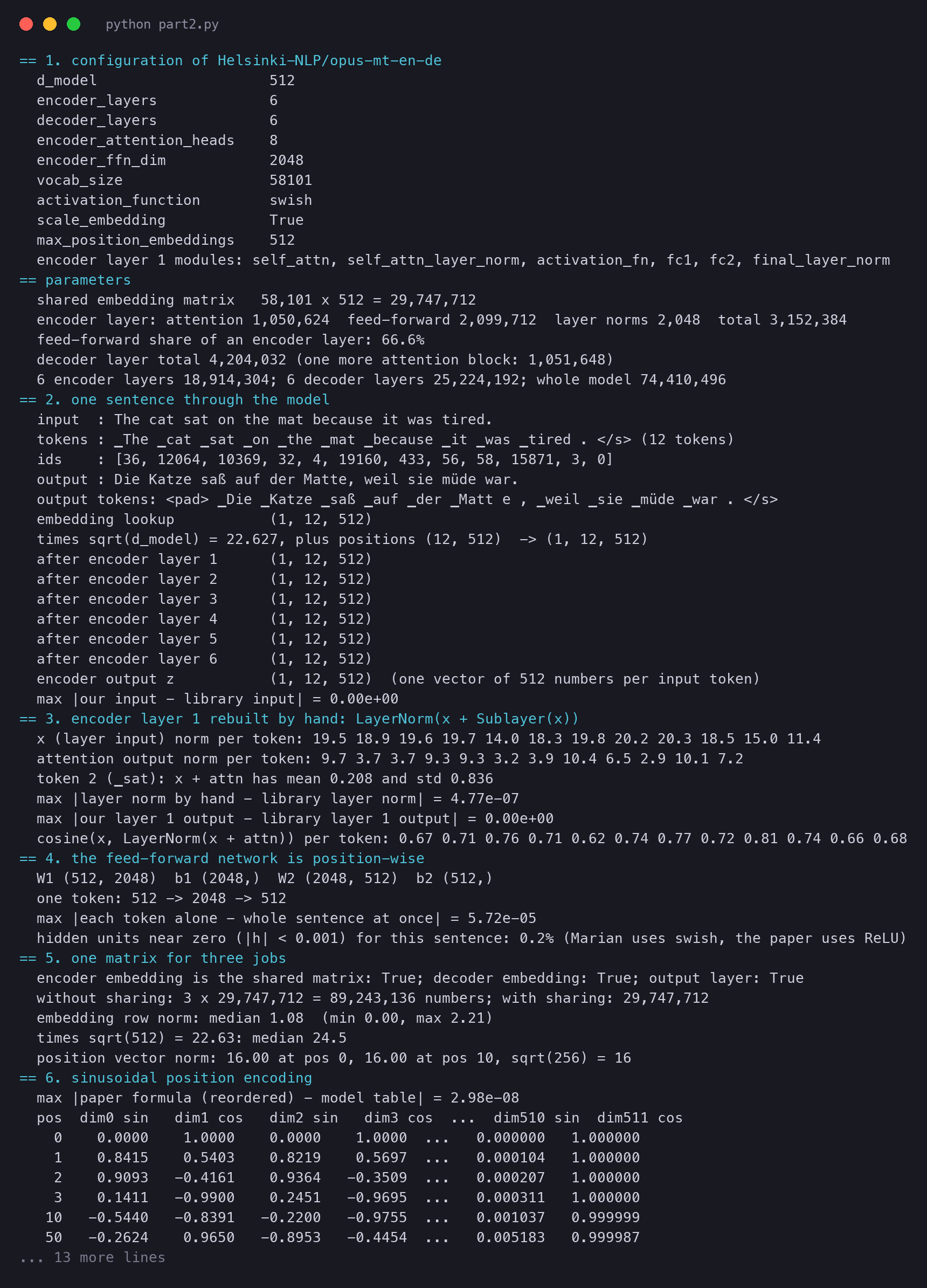

Terminal output of tx_part2.py: the configuration and weight counts, the translation of one sentence, the shapes through the encoder, layer 1 rebuilt by hand, the feed-forward and shared-table checks, and the position encoding table — The first part of the output of tx_part2.py, as it ran for this article.

The paper and the code

Attention Is All You Need (NeurIPS 2017) · official code (tensor2tensor) · our scripts for this part

The Architecture: Stacks, Feed-Forward Layers and Positions

An encoder and a decoder#

Our model and one sentence#

Figure 1: the whole model in one picture#

The encoder stack#

The residual connection#

The residual wrapper in code#

Layer normalization#

Layer normalization in code#

The decoder stack#

The feed-forward network#

The feed-forward network in code#

Embeddings and the shared matrix#

Why multiply by dmodel\sqrt{d_{\text{model}}}dmodel​​?#

The embedding and the output layer in code#

Positional encoding#

Why a shift is a rotation#

The position encoding in code#

One encoder layer from our own pieces#

The whole encoder#

What goes wrong when one detail is missing#

What our model cannot show#

The paper and the code#

An encoder and a decoder

Our model and one sentence

Figure 1: the whole model in one picture

The encoder stack

The residual connection

The residual wrapper in code

Layer normalization

Layer normalization in code

The decoder stack

The feed-forward network

The feed-forward network in code

Embeddings and the shared matrix

Why multiply by $\sqrt{d_{\text{model}}}$ ?

The embedding and the output layer in code

Positional encoding

Why a shift is a rotation

The position encoding in code

One encoder layer from our own pieces

The whole encoder

What goes wrong when one detail is missing

What our model cannot show

The paper and the code