Transformer, explained · Part 1 of 7 · Covers Title, Abstract, §1, §2

The Big Idea: Attention Is All You Need

Why the best translation models of 2016 were slow to train, and the claim that attention alone can replace them. We read the title, the abstract and the first two sections, and we run a released Transformer that translates English into German.

Attention Is All You Need. Ashish Vaswani, Noam Shazeer, Niki Parmar, Jakob Uszkoreit, Llion Jones, Aidan N. Gomez, Łukasz Kaiser, Illia Polosukhin. NeurIPS 2017, 2017. arXiv:1706.03762

In June 2017, a team from Google put a short paper on arXiv. It described a translation model that reads a whole sentence in one step. The best models of the time read it one word after the other. The model is the Transformer, and its design now runs almost every large language model.

Each piece below shows the exact lines of the paper, then explains them.

The title

From the paperTitle

What it says

"Attention Is All You Need."

What it means

The title is a claim, and a bold one. In 2017, a translation model was a large machine with many parts. Recurrent layers read the words in order. Convolutional layers looked at small windows of words. An attention step helped the two halves of the model talk to each other. Attention was a helper part, added to a recurrent network.

The title says that the helper can do the whole job. Remove the recurrent layers and the convolutions, keep attention, and the model gets better and faster. The rest of the paper is the evidence for this claim.

The word "need" is also exact. The paper does not say that attention is the best part of a model. It says that the other parts are not necessary. The model still has small feed-forward layers and some other pieces (Part 2 shows all of them). But the only step that moves information between words is attention.

The abstract

From the paperAbstract

What it says

"The dominant sequence transduction models are based on complex recurrent or convolutional neural networks that include an encoder and a decoder. The best performing models also connect the encoder and decoder through an attention mechanism."

What it means

"Sequence transduction" is a long name for a familiar job: a sequence goes in, and a different sequence comes out. Translation is the main example. "The dog sat on the mat" goes in, and "Der Hund saß auf der Matte" comes out. The two sentences can have different lengths and a different word order.

The first sentence describes the standard machine for this job in 2017. An encoder reads the input sentence and turns it into numbers. A decoder reads those numbers and writes the output sentence, one word at a time. Both halves were recurrent or convolutional networks. The Background page explains both kinds.

The second sentence names the best version of that machine. Its decoder does not only get one summary of the input. At each output word, it looks back at all the input words and decides which ones matter now. That look-back is the attention step, and it came from translation research in 2014 and 2015.

From the paperAbstract

What it says

The paper proposes "the Transformer, based solely on attention mechanisms, dispensing with recurrence and convolutions entirely". On two translation tasks, the models are "superior in quality while being more parallelizable and requiring significantly less time to train".

What it means

This is the big idea in one sentence. Keep the encoder and the decoder. Keep attention. Remove the recurrent layers and the convolutions. Attention is no longer a bridge between two recurrent networks. It is the material of the whole building.

The second sentence makes two claims, and both are surprising. Usually, a faster model is a worse model, and you pay for speed with quality. Here the paper claims better translations and a shorter training time at the same moment.

"More parallelizable" is the reason for the speed. A recurrent network must finish word 1 before it can start word 2. Attention has no such order, so a GPU can process all the words of a sentence at the same time. The next section of this page shows why, and our run measures it.

From the paperAbstract

$The results sentences of the abstract, with 28.4 BLEU, by over 2 BLEU, 41.8, 3.5 days on eight GPUs and small fraction of the training costs highlighted$

What it says

The model gets "28.4 BLEU on the WMT 2014 English-to-German translation task", better than the best earlier results, "including ensembles, by over 2 BLEU". On English-to-French, it gets "41.8 after training for 3.5 days on eight GPUs, a small fraction of the training costs of the best models from the literature".

What it means

BLEU is the score that translation research uses (the yellow box below explains it). WMT 2014 is a public competition with fixed training data and fixed test sentences, so all teams measure on the same sentences. A gain of 2 BLEU on a mature benchmark is a large step.

The word "ensembles" matters. An ensemble is several models that vote on each translation. Ensembles score higher than one model, but they cost several times more to train and to run. A single Transformer beat the earlier ensembles on English-to-German.

The last claim is about cost. Eight GPUs for 3.5 days is a modest budget for a model that sets a new record. Part 6 reads Table 2 of the paper, which compares the training cost of each model in floating-point operations.

From the paperAbstract

What it says

"We show that the Transformer generalizes well to other tasks by applying it successfully to English constituency parsing both with large and limited training data."

What it means

A new model that wins on one task can be a lucky fit for that task. So the paper tries a second task that is very different from translation. In constituency parsing, the input is a sentence and the output is its grammar tree. The tree shows which words form a phrase, and how the phrases nest.

"Limited training data" is the hard test. Large models with few examples often memorise the examples and fail on new sentences. The paper reports that the Transformer did well in both settings. Part 6 reads the numbers. This sentence was the first hint that the design is general, and the years after 2017 confirmed it.

A released Transformer, translating one sentence

The paper's own weights are not on the public model hubs. So we use a released model with the same shapes as the paper's base model: Helsinki-NLP/opus-mt-en-de, a Transformer (MarianMT) that translates English into German. Our script loads it and translates one sentence:

plain text

== 1. A released Transformer: Helsinki-NLP/opus-mt-en-de
encoder layers 6, decoder layers 6, d_model 512, heads 8, d_ff 2048, vocabulary 58,101
parameters: 74,410,496
English: The dog sat on the mat because it was tired.
source tokens (12): ['▁The', '▁dog', '▁sat', '▁on', '▁the', '▁mat', '▁because', '▁it', '▁was', '▁tired', '.', '</s>']
German : Der Hund saß auf der Matte, weil er müde war.
output tokens (15): ['<pad>', '▁Der', '▁Hund', '▁saß', '▁auf', '▁der', '▁Matt', 'e', ',', '▁weil', '▁er', '▁müde', '▁war', '.', '</s>']

The shapes match the base model of the paper. It has 6 encoder layers and 6 decoder layers, with vectors of 512 numbers. It has 8 attention heads and 2,048 numbers inside each feed-forward layer. Part 2 explains each of these numbers. The English sentence becomes 12 tokens. The mark "▁" means "a space comes before this token", and </s> marks the end of the sentence.

The translation is correct, and one detail shows real understanding. In German, "Hund" (dog) is masculine and "Matte" (mat) is feminine. So "it" becomes "er" for the dog and "sie" for the mat. The model wrote "er": it linked "it" with "dog", six words earlier, and not with the closer "mat". This kind of link between distant words is what the rest of this page is about.

This model is not the paper's model. Marian was trained later, on different data, with its own vocabulary. It shows the design and the shapes, not the paper's BLEU scores.

The problem with recurrence

From the paper§1

What it says

"Recurrent neural networks, long short-term memory [13] and gated recurrent [7] neural networks in particular, have been firmly established as state of the art approaches in sequence modeling and transduction problems such as language modeling and machine translation."

What it means

The introduction starts with the opponent. In 2017, the recurrent network was the standard tool for text. The LSTM (1997) and the GRU (2014) are improved recurrent networks that remember information over more words. Google's own translation service used a large LSTM model in 2016.

"Firmly established" tells you how big the claim of the title is. The paper does not attack a weak method. It attacks the method that every strong system of the time used. To replace it, the new model must be better on the same tasks, and the paper must show it with numbers.

From the paper§1

What it says

Recurrent models "generate a sequence of hidden states $h_t$ , as a function of the previous hidden state $h_{t-1}$ and the input for position $t$ ". "This inherently sequential nature precludes parallelization within training examples." Tricks have made recurrent models faster, but "the fundamental constraint of sequential computation, however, remains."

What it means

This paragraph is the heart of the paper's argument. Think of a line of people who pass a message by whispering. Person 5 cannot start before person 4 finishes. A hundred people in the line need a hundred turns, and more people do not shorten the line.

A recurrent network is that line. To compute the state of word 5, it needs the state of word 4. So a sentence of 50 words needs 50 steps, one after the other, even on a GPU with thousands of cores. "Within training examples" is the exact point. The GPU can still work on many sentences at the same time, but not on the words of one sentence.

Why not just process more sentences at the same time? The paper answers: "memory constraints limit batching across examples". Each sentence in a batch needs memory for all its hidden states. Long sentences fill the memory of the GPU quickly. So the number of sentences in a batch is limited, and the GPU waits.

The paper writes the recurrence in words. In symbols, it is this:

h_t = f(h_{t-1},\, x_t)

Read it from left to right. $h_t$ is the hidden state after word $t$ , a vector. $h_{t-1}$ is the hidden state after the word before. $x_t$ is the vector of word $t$ . $f$ is a function with learned weights, the same function at every step. The arrow of time is inside the formula: you cannot compute $h_t$ before you have $h_{t-1}$ .

The most basic recurrent network uses this $f$ :

h_t = \tanh\left(W h_{t-1} + U x_t\right)

Here $W$ and $U$ are learned matrices, and $\tanh$ squeezes each number into the range from -1 to 1. To see the problem with long sentences, shrink everything to one number. Let $W = 0.5$ , $U = 1$ and $h_0 = 0$ . The first word has the value 1, and every later word has the value 0. Our script follows the trace of the first word:

plain text

== 2. The recurrence h_t = tanh(w * h_(t-1) + u * x_t), with w = 0.5, u = 1.0, h_0 = 0
  t=1: x=1  h = tanh(0.5 x 0.0000 + 1.0 x 1) = tanh(1.0000) = 0.7616
  t=2: x=0  h = tanh(0.5 x 0.7616 + 1.0 x 0) = tanh(0.3808) = 0.3634
  t=3: x=0  h = tanh(0.5 x 0.3634 + 1.0 x 0) = tanh(0.1817) = 0.1797
  t=4: x=0  h = tanh(0.5 x 0.1797 + 1.0 x 0) = tanh(0.0899) = 0.0896
  t=5: x=0  h = tanh(0.5 x 0.0896 + 1.0 x 0) = tanh(0.0448) = 0.0448
  t=6: x=0  h = tanh(0.5 x 0.0448 + 1.0 x 0) = tanh(0.0224) = 0.0224
  the trace of word 1 shrinks by about half at each step: it must pass through every later state

Check the first line by hand: $0.5 \times 0 + 1 \times 1 = 1$ , and $\tanh(1) = 0.7616$ . At each later step, the old value is multiplied by 0.5, so the trace of word 1 halves. After five more words, only 0.0224 is left. Real networks have learned weights and gates, and the LSTM was designed to slow this fading. But two facts stay: word 1 reaches word 6 only through all the states between them, and the six steps must run in order.

Top: a recurrent network computes the states h1 to h6 one after the other, so the first word reaches h6 only through five later states. Bottom: self-attention computes six new vectors together, and each one reads all six words directly. The highlighted lines show the six links of the last word.

The loop and the matrix product, in code

The figure is the whole argument of §1, and it fits in two short functions. The first is a recurrent layer, our Method 1. Read the for line: step t uses h, and h is the result of step t - 1. There is no way to start step 5 before step 4 is done.

python

def rnn_layer(X, W, U, b):
    """Method 1: a recurrent layer. X is (batch, n, d). Step t cannot start before step t - 1 ends."""
    B, n, d = X.shape
    h = torch.zeros(B, d)                               # h_0
    states = []
    for t in range(n):                                  # n steps, one after the other
        h = torch.tanh(X[:, t] @ W.T + h @ U.T + b)     # (B, d): needs the h of the step before
        states.append(h)
    return torch.stack(states, 1)                       # (B, n, d)

The second is self-attention in its most basic form, with no learned weights: each word is its own query, key and value. Part 3 adds the learned matrices and the heads. Here we only need the shape of the computation. There is no loop over words. One matrix product compares every word with every word, a softmax turns each row into weights, and a second product mixes the words.

python

def attention_layer(X):
    """Method 1: self-attention with no learned weights, Q = K = V = X. All n rows in one go."""
    d = X.shape[-1]
    scores = X @ X.transpose(1, 2) / math.sqrt(d)      # (B, n, n): every word against every word
    weights = torch.softmax(scores, dim=-1)             # each row adds up to 1
    return weights @ X                                  # (B, n, d): a weighted mix for every word at once

Follow the shapes for a batch of 32 sentences of 12 words, each word a vector of 512 numbers. X has the shape (32, 12, 512). X.transpose(1, 2) swaps the last two axes, so it has the shape (32, 512, 12). Their product has the shape (32, 12, 12): for each sentence, a table of 12 × 12 scores. The division by $\sqrt{d}$ keeps the scores in a useful range; Part 3 explains it.

Our Method 2 is the library: nn.RNN for the loop, with the same weights, and F.scaled_dot_product_attention, the attention function that PyTorch ships. We also run two small tests. First, we compute row 7 of the attention output alone. Second, we change only word 3 and measure how much each output moves.

python

# Each attention row needs only X, not the other outputs: compute row 7 alone.
with torch.no_grad():
    row7 = torch.softmax(X[:, 7:8] @ X.transpose(1, 2) / math.sqrt(d), -1) @ X     # (B, 1, d)
log(f'  attention row 7 computed alone, from X only: max |row 7 alone - row 7 of the full product| = {diff(row7[:, 0], A_ours[:, 7]):.1e}')

# Change word 3 only, and see which outputs move. Small word vectors keep the attention weights spread out.
with torch.no_grad():
    Xs = 0.05 * torch.randn(B, n, d)                    # (B, 12, 512)
    Xs2 = Xs.clone(); Xs2[:, 3] += 0.05                 # the same sentence, word 3 changed
    move_rnn = (rnn_layer(Xs2, W, U, b) - rnn_layer(Xs, W, U, b)).abs().amax(dim=(0, 2))   # (12,): one number per output
    move_att = (attention_layer(Xs2) - attention_layer(Xs)).abs().amax(dim=(0, 2))

plain text

== 1. Sequential against parallel (width d = 512, batch 32)
  X (32, 12, 512)
  RNN loop: 12 steps in order -> (32, 12, 512); max |ours - nn.RNN| = 8.3e-07
  attention: 1 product X X^T (32, 12, 12), softmax, 1 product with X -> (32, 12, 512); max |ours - F.scaled_dot_product_attention| = 1.2e-07
  attention row 7 computed alone, from X only: max |row 7 alone - row 7 of the full product| = 0.0e+00
  change word 3 only; largest change of each output 0..11:
    RNN       0.000 0.000 0.000 0.089 0.053 0.031 0.016 0.013 0.005 0.003 0.002 0.001
    attention 0.004 0.004 0.004 0.006 0.004 0.004 0.004 0.004 0.004 0.004 0.004 0.004

Both of our functions agree with the library to less than one millionth. Now read the last four lines, because they are the point of §1.

Row 7 of attention, computed alone, is exactly row 7 of the full product. It needs only the inputs X, not any other output. So the 12 rows can go to 12 groups of GPU cores at the same time. The RNN has no such row: $h_7$ needs $h_6$ , which needs $h_5$ , and so on.

The change test shows the two kinds of path. In the RNN, outputs 0 to 2 do not move at all, because they were computed before word 3. Output 3 moves by 0.089, and then the change fades along the chain: 0.053, 0.031, and only 0.001 at output 11. That is the fading trace of the Background page, in a real layer of 512 numbers.

In attention, every output moves, even outputs 0, 1 and 2, which come before word 3. The change reaches output 11 as strongly as output 0, because each output reads word 3 directly, in one step. Output 3 moves a little more, because word 3 is also its own query.

A learner often reads "parallel" as "no dependencies at all". That is wrong. Each attention output depends on every input word, as the second row shows. What attention removes is the dependence of one output on another output. All the inputs are known at the start, so all the outputs can start at once.

How long does each take on a laptop CPU? The script times all four versions, with 16, 64 and 256 words:

python

def fastest(f, k=10):
    f()
    best = 1e9
    for _ in range(k):
        t0 = time.perf_counter(); f(); best = min(best, time.perf_counter() - t0)
    return best * 1000

plain text

   time on the CPU (4 threads), forward pass only, fastest of 10 runs, random weights
     n  steps in order  our loop ms  nn.RNN ms  our attention ms  SDPA ms
    16         16 vs 1          2.1        1.8               0.3      0.1
    64         64 vs 1          9.0        7.4               0.7      0.5
   256        256 vs 1         51.9       38.2               7.9      4.3

We take the fastest of 10 runs, because a slow run usually means that the computer did something else at that moment. The library's nn.RNN is faster than our loop, because its loop is written in C++. But it still takes 256 steps in order for 256 words. Our attention and the library's SDPA (scaled dot-product attention) take one step of matrix products at every length.

Keep the warnings in mind. These are untrained layers with no learned query, key and value matrices, on a CPU with 4 threads. The times change from run to run. And attention's work grows with $n^2$ : at 256 words, the score table has 256 × 256 entries for each sentence. The next table shows what happens on a GPU and at 1,024 words.

Real layers on a laptop GPU

How much does the order cost with real layers on a GPU? We timed one GRU layer and one self-attention layer, both with vectors of 512 numbers, on batches of 32 random sentences. The GRU is a recurrent layer with gates, a lighter cousin of the LSTM. The attention layer is PyTorch's nn.MultiheadAttention, with learned matrices and 8 heads. The script tx_part1.py also writes the GRU as the loop that it is:

python

def gru_loop(x):
    """The GRU of §1, written as the loop that it is: step t needs h_(t-1)."""
    cell = torch.nn.GRUCell(d, d)
    cell.weight_ih, cell.weight_hh, cell.bias_ih, cell.bias_hh = gru.weight_ih_l0, gru.weight_hh_l0, gru.bias_ih_l0, gru.bias_hh_l0
    h = torch.zeros(x.shape[0], d)
    for t in range(x.shape[1]):
        h = cell(x[:, t], h)
    return h

The cell gets the weights of the full GRU layer, and the for loop takes one word per step. The output:

plain text

== 3. One GRU layer (a loop over the words) against one self-attention layer (all words at once)
   width 512, batch 32, device mps (Apple M5 Pro laptop GPU), forward pass only, fastest of 20 runs
 words n  GRU steps   GRU ms  attention steps  attention ms  GRU / attention
      16         16      2.3                1           0.7             3.3x
      64         64      6.8                1           2.0             3.4x
     256        256     18.4                1           4.8             3.8x
    1024       1024     75.5                1          39.1             1.9x
check: the library GRU equals our step-by-step loop, max difference 3.3e-07

The GRU needs $n$ steps in order; the attention layer needs one. On our laptop GPU, the attention layer was 1.9 to 3.8 times faster at every length.

The last line checks that the library GRU is the loop that we wrote by hand. The two results differ by less than one part in a million.

This table needs two warnings. First, attention is not free. Each word compares itself with every other word, so the work grows with $n^2$ , and the gap gets smaller at 1,024 words. Part 4 counts this cost exactly.

Second, these are single layers with random weights, timed on a laptop while other jobs ran. The ratio jumps from run to run. The table shows the shape of the problem, not the paper's training speed-up.

Training is parallel, writing is not

There is a subtle point that the abstract does not say. The Transformer's decoder still writes a translation one token at a time, because each new word depends on the words before it. The parallel speed-up is in training. During training, the correct German sentence is known in advance, so the model can predict every position at the same time. This trick is teacher forcing.

plain text

== 4. Marian: score a known German sentence in one call, or write it one token per call
German tokens m = 14
teacher forcing: 1 decoder call gives logits of shape (1, 14, 58101) (one row per position), 67 ms
  the 14 predicted tokens equal the generated ones: True; mean loss 0.203
generation: 14 decoder calls, one per token, 146 ms

With the known German sentence of 14 tokens, one call of the decoder gives 14 rows of scores, one row for each position. Each row has 58,101 scores, one for each token in the vocabulary. The best token in each row is exactly the token that the model generated. Writing the same sentence from nothing needed 14 calls, one after the other. A recurrent decoder needs the loop in both cases; the Transformer needs it only when it writes.

Teacher forcing in code

The table above came from one line, model(**enc, labels=labels), and the library hid the work. Here we do each step ourselves with the same released model, so that nothing is hidden. The German sentence is the model's own translation of our English sentence: 14 tokens, the last one </s>.

Step 1: shift the sentence. At position $t$ , the decoder must predict token $t$ of the German sentence. So its input at position $t$ must be the token before it. We build the input by putting a start token in front and dropping the last token:

python

start = torch.tensor([[cfg.decoder_start_token_id]])          # Marian uses <pad> (id 58100) as the start token
dec_in = torch.cat([start, labels[:, :-1]], dim=1)            # (1, m): drop the last token, put start in front
dec_lib = shift_tokens_right(labels, cfg.pad_token_id, cfg.decoder_start_token_id)

labels[:, :-1] takes every token except the last one. The library has a function for this step, shift_tokens_right, and we compare with it.

Step 2: one call for all positions. We give the model the English ids and the whole shifted German input at once:

python

with torch.no_grad():
    out = model(**src, decoder_input_ids=dec_in)
logits = out.logits                                           # (1, m, 58101): one row of scores per position

Step 3: the loss by hand. The loss is the next-token loss of the Background page: $-\log p$ of the right token, averaged over the positions.

\text{loss} = -\frac{1}{m} \sum_{t=0}^{m-1} \log p\left(y_t \mid y_{<t},\ \text{English}\right)

Here $m = 14$ is the number of German tokens, $y_t$ is the right token at position $t$ , and $y_{<t}$ are the tokens before it. In code, log_softmax turns each row of scores into log-probabilities. Then we pick, in each row, the entry of the right token:

python

logp = torch.log_softmax(logits, dim=-1)                      # (1, m, 58101)
logp_right = logp[0, torch.arange(m), labels[0]]              # (m,): log p of the right token at each position
loss_ours = -logp_right.mean()
with torch.no_grad():
    loss_lib = model(**src, labels=labels).loss               # Method 2: the library shifts and averages for us

The line with torch.arange(m) is the one that needs a second look. It picks one number from each row: row 0 at column labels[0, 0], row 1 at column labels[0, 1], and so on. The result is 14 log-probabilities, one per position. Here is the output, with a table of what the decoder reads and what it must predict at each position:

plain text

== 2. Teacher forcing with Helsinki-NLP/opus-mt-en-de
  English ids (1, 12); German labels (1, 14): ['▁Der', '▁Hund', '▁saß', '▁auf', '▁der', '▁Matt', 'e', ',', '▁weil', '▁er', '▁müde', '▁war', '.', '</s>']
  decoder input (1, 14): ['<pad>', '▁Der', '▁Hund', '▁saß', '▁auf', '▁der', '▁Matt', 'e', ',', '▁weil', '▁er', '▁müde', '▁war', '.']
  same as the library shift_tokens_right: True
  one call: logits (1, 14, 58101)
  loss by hand 0.2030; library loss 0.2030; difference 1.5e-08
  pos   decoder reads   must predict  p(right)   top guess
    0           <pad>           ▁Der     0.796        ▁Der
    1            ▁Der          ▁Hund     0.946       ▁Hund
    2           ▁Hund           ▁saß     0.723        ▁saß
    3            ▁saß           ▁auf     0.782        ▁auf
    4            ▁auf           ▁der     0.767        ▁der
    5            ▁der          ▁Matt     0.915       ▁Matt
    6           ▁Matt              e     0.914           e
    7               e              ,     0.771           ,
    8               ,          ▁weil     0.837       ▁weil
    9           ▁weil            ▁er     0.565         ▁er
   10             ▁er          ▁müde     0.830       ▁müde
   11           ▁müde           ▁war     0.881        ▁war
   12            ▁war              .     0.900           .
   13               .           </s>     0.889        </s>
  top guess equals the label at 14 of 14 positions

Read the table diagonally. The token that position 1 must predict, ▁Hund, is the token that position 2 reads. Each row sees only the tokens above it. Our loss, 0.2030, equals the library's loss and the 0.203 of the earlier run.

The lowest probability is 0.565, for "er" at position 9. That is the word whose gender depends on "dog", six words back. The model is right, but less sure than anywhere else in the sentence. Hard links between distant words are the hard part of translation.

Why does this need a mask? Position 3 reads ▁saß, and it must predict ▁auf. But ▁auf is also in the input, at position 4. Without a mask, position 3 could look one place to the right and copy the answer. The loss would be almost 0, and the model would learn nothing useful. The decoder's mask hides the later positions, so each row must really predict.

Writing: one decoder call per token

When the model translates a new sentence, it does not have the German sentence. It must write it. Here is the generation loop written out, our Method 1:

python

def greedy(model, src, max_new=40):
    """Method 1: our own generation loop. The encoder runs once; the decoder runs once per new token."""
    enc_out = model.get_encoder()(**src)                      # (1, 12, 512), reused at every step
    ys = torch.tensor([[cfg.decoder_start_token_id]])         # (1, 1): only the start token
    step_logits = []
    for _ in range(max_new):
        logits = model(encoder_outputs=enc_out, attention_mask=src.attention_mask, decoder_input_ids=ys).logits
        last = logits[:, -1].clone()                          # (1, 58101): scores for the next token only
        last[:, cfg.pad_token_id] = -float('inf')             # never write the start/pad token (generate does the same)
        nxt = last.argmax(-1, keepdim=True)                   # (1, 1): the most likely token
        step_logits.append(logits[0, -1])
        ys = torch.cat([ys, nxt], dim=1)                      # feed it back in: the input grows by one
        if nxt.item() == cfg.eos_token_id:
            break
    return ys, torch.stack(step_logits)

The encoder runs once, and its 12 vectors are kept. The decoder runs inside the loop. At each step, it reads all the tokens so far, and we keep only the scores of the last position. We pick the best token and append it, so ys grows from shape (1, 1) to (1, 2), (1, 3) and so on. The loop is the same chain as in a recurrent network: step 5 needs the token of step 4.

Method 2 is the library's model.generate with one beam and no sampling, which is greedy decoding. We compare the two outputs, and we also compare the scores of our loop with the teacher-forced scores of Step 2:

plain text

== 3. Writing the translation: our greedy loop against model.generate
  ours    : Der Hund saß auf der Matte, weil er müde war.  (14 decoder calls)
  generate: Der Hund saß auf der Matte, weil er müde war.
  same tokens: True
  max |teacher-forced logits - loop logits at the same position| = 1.0e-05

Our loop and the library write the same 14 tokens. The last line is the important one. The scores that the loop computed one step at a time equal the scores of the single teacher-forced call, to 0.00001. So the one parallel call computes exactly what 14 separate calls compute. This is why the Transformer can train on all positions at once and still learn the same thing that it does when it writes.

Our loop is slow on purpose: at every step, it runs the decoder again over all the earlier tokens. Real code keeps the keys and values of earlier positions in a cache, so each step only computes the new position. That makes each step cheaper, but the steps still run in order.

From the paper§1

What it says

Attention mechanisms allow "modeling of dependencies without regard to their distance in the input or output sequences". But "in all but a few cases", they "are used in conjunction with a recurrent network".

What it means

Here is the good news that sits next to the bad news. In a recurrent network, word 1 reaches word 30 only through 29 states, and the signal fades on the way. Attention has no such road. When the decoder writes a word, it can look straight at any input word, the first one or the last one, at the same cost.

A dependency is a link between two words that the model must get right. "It" depends on "dog" in our example, because the dog decides the gender of "er". Some dependencies span many words, for example a verb at the end of a long German sentence.

The last sentence names the strange situation of 2017. The strong part, attention, was used as an addition to the weak part, the recurrent network. The loop was still there, and so was its speed limit. The next paragraph draws the obvious conclusion.

From the paper§1

What it says

The Transformer is "a model architecture eschewing recurrence and instead relying entirely on an attention mechanism to draw global dependencies between input and output". It reaches a new state of the art "after being trained for as little as twelve hours on eight P100 GPUs".

What it means

"Eschewing" means "keeping away from". The paper removes the loop completely. Every link between words, inside the input, inside the output and between the two, goes through attention. "Global" means that each word can reach every other word in the sentence, not only its neighbours.

Twelve hours on eight GPUs is the training time of the smaller base model (§5.2 gives it, and Part 5 reads it). The P100 was a strong NVIDIA data-centre GPU in 2016. Earlier top systems, such as Google's LSTM translation model of 2016, trained for days on many more GPUs. So the claim is not "slightly faster". It is a model that a single machine can train overnight.

The models that came closest

The second section of the paper is short. It names the models that had already tried to remove the loop, and it says why they were not enough.

From the paper§2

What it says

The Extended Neural GPU, ByteNet and ConvS2S use convolutional networks, "computing hidden representations in parallel for all input and output positions". But the number of operations to relate two positions "grows in the distance between positions, linearly for ConvS2S and logarithmically for ByteNet". In the Transformer, it is "a constant number of operations", at the cost of "reduced effective resolution", which "Multi-Head Attention" counteracts.

What it means

Convolutional models had already solved the speed problem. A convolution looks at a small window of neighbouring words, and it can process all the windows of a sentence at the same time. So these models trained in parallel, like the Transformer.

Their weakness is reach. One layer with a window of 3 words links each word only with its close neighbours. To connect two words far apart, the signal must climb through many layers, like news that travels from village to village. ConvS2S needs more layers in proportion to the distance. ByteNet spaces its windows wider in each layer, so it needs fewer layers, but the number still grows. The paper cites earlier work: the longer this path, the harder it is to learn the link.

In the Transformer, any two words are one attention step apart. The cost is a blur. Attention mixes many words into one weighted average, and an average loses detail. Imagine that "it" needs "dog" for its gender and "tired" for its meaning. One average of the two is neither. The fix is several attention steps side by side, each free to look at a different word: multi-head attention, which Part 3 explains.

How many layers does a signal climb? Take a causal convolution of width $k$ , as in ConvS2S's decoder: each layer reaches $k - 1$ more words back. With $L$ layers, the reach is $L(k-1)$ words. Now take ByteNet-style dilated layers of width 2, with gaps of 1, 2, 4, 8 words: the reach after $L$ layers is $1 + 2 + 4 + \dots + 2^{L-1} = 2^L - 1$ . To link two words $d$ positions apart, the number of layers is:

L_{\text{conv}} = \left\lceil \frac{d}{k-1} \right\rceil, \qquad L_{\text{dilated}} = \left\lceil \log_2 (d+1) \right\rceil, \qquad L_{\text{attention}} = 1

The brackets $\lceil \cdot \rceil$ round up to the next whole number. A worked case: $d = 10$ and $k = 3$ give $\lceil 10 / 2 \rceil = 5$ convolution layers and $\lceil \log_2 11 \rceil = \lceil 3.46 \rceil = 4$ dilated layers. A recurrent network needs 10 steps. Our script prints the table for four distances:

plain text

== 5. Layers a signal crosses between two words d positions apart
   ConvS2S: kernel width 3, each layer reaches 2 more words back; ByteNet: kernel width 2, dilations 1, 2, 4, ...
    d  recurrent  ConvS2S  ByteNet  self-attention
    2          2        1        2               1
   10         10        5        4               1
   50         50       25        6               1
  200        200      100        8               1

At 200 words apart, a recurrent network needs 200 steps and a ConvS2S-style stack needs 100 layers. The dilated stack needs 8. Self-attention needs 1 at every distance. These are idealised counts for one layout of each model; the real ConvS2S and ByteNet use other widths. Part 4 reads the paper's own table of these costs, Table 1.

From the paper§2

What it says

"Self-attention, sometimes called intra-attention is an attention mechanism relating different positions of a single sequence in order to compute a representation of the sequence."

What it means

In translation attention, the decoder looks at the encoder: a German word looks at English words. That is attention between two sequences. Self-attention turns the look inward. The words of one sentence look at the other words of the same sentence.

Why look inward? Because the meaning of a word depends on its neighbours. "Bank" next to "river" is not "bank" next to "money". After one step of self-attention, the vector of "bank" carries some of the vector of "river". It becomes a vector for "bank in this sentence". That is what "a representation of the sequence" means: one vector for each word, in its context.

The idea was not new. The paper lists earlier uses in reading comprehension, summaries and sentence vectors. What was new is the next paragraph.

From the paper§2

What it says

"the Transformer is the first transduction model relying entirely on self-attention to compute representations of its input and output without using sequence-aligned RNNs or convolution."

What it means

This sentence states what is new, and it is careful. Attention was not new. Self-attention was not new. What was new is a full translation model, encoder and decoder, with no recurrent layer and no convolution at all.

"Sequence-aligned" is the precise word for the loop. A recurrent network aligns its computation with the order of the words: step 1 for word 1, step 2 for word 2. The Transformer drops this alignment.

But word order still matters in language, and attention by itself ignores it. "dog bites man" and "man bites dog" contain the same words. So the model must get the order from somewhere else. Part 2 shows the answer: position encodings, added to each word vector.

Key takeaways

The claim: a translation model needs no recurrent layers and no convolutions. Attention alone can move all the information between words.
Sequence transduction turns one sequence into another, for example English into German. An encoder reads the input, and a decoder writes the output one token at a time.
The problem with recurrence: $h_t = f(h_{t-1}, x_t)$ . Each state waits for the one before it, so the words of one sentence cannot be processed in parallel. In our one-number example, the trace of word 1 fell from 0.7616 to 0.0224 in six steps.
On our laptop GPU, one self-attention layer was 1.9 to 3.8 times faster than one GRU layer for 16 to 1,024 words. Attention's work grows with $n^2$ , which Part 4 counts.
Training is parallel, writing is not: with teacher forcing, Marian scored a 14-token German sentence in 1 decoder call. Writing it took 14 calls.
In code, the two claims are a few lines each. Each attention row needs only the inputs, so all rows can start together; each RNN state needs the state before it. Our teacher-forced loss (0.2030) equals the library's, and our 14-call greedy loop gives the same scores as the single call, to 0.00001.
Path length: between two words 200 positions apart, a recurrent network needs 200 steps, a width-3 convolution stack 100 layers and a dilated stack 8. Self-attention needs 1.
The price of one-step links is a blur from averaging. Multi-head attention fixes it.
The results: 28.4 BLEU on WMT 2014 English-to-German, over 2 BLEU above the best earlier results, ensembles included. 41.8 BLEU on English-to-French after 3.5 days on 8 GPUs.
A released model with the paper's base shapes (opus-mt-en-de: 6 + 6 layers, d_model 512, 8 heads, d_ff 2048) has 74.4 million parameters. It chose "er" for "it", which links "it" to the dog.

Next, in Part 2: §3 and Figure 1 of the paper, the architecture. Part 2 opens the encoder and the decoder and follows each shape through the released model. It covers the residual connections, layer normalisation, the feed-forward layers, the embeddings and the position encodings.

Run it yourself

The script behind this part is code/papers/transformer/tx_part1.py. It loads the released translation model and translates one sentence. It works the recurrence by hand and times a GRU layer against an attention layer. It also compares teacher forcing with generation, and prints the path lengths. Every number is saved in results/part1.json. The second script, tx_part1_scratch.py, holds the code of the sections "The loop and the matrix product, in code", "Teacher forcing in code" and "Writing: one decoder call per token".

bash

pip install torch transformers sentencepiece
python tx_part1.py           # downloads Helsinki-NLP/opus-mt-en-de (about 300 MB)
python tx_part1_scratch.py   # the loop and the matrix product, teacher forcing and the greedy loop by hand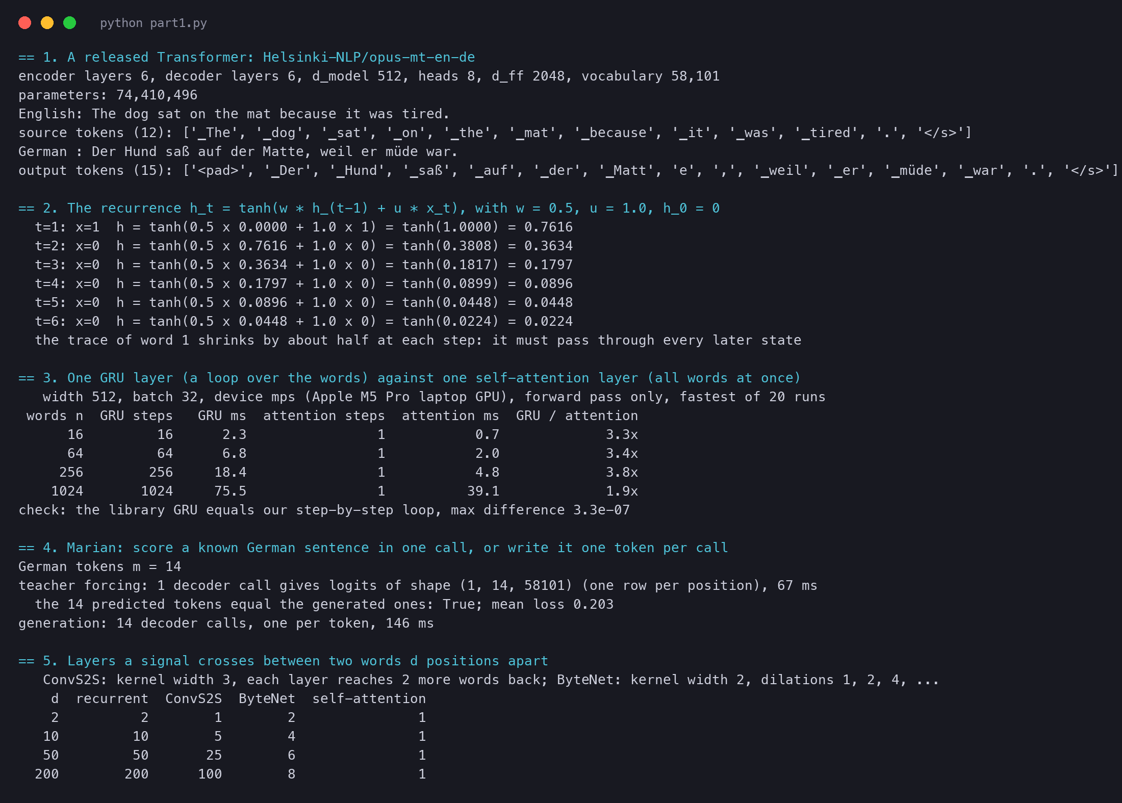

Terminal output of tx_part1.py: the shapes of the released model and its translation, the recurrence worked by hand, the GRU and attention timing table, teacher forcing against generation, and the path-length table — The full output of tx_part1.py, as it ran for this article.

The paper and the code

Attention Is All You Need (NeurIPS 2017) · official code (tensor2tensor) · our scripts for this part

The Big Idea: Attention Is All You Need

The title#

The abstract#

A released Transformer, translating one sentence#

The problem with recurrence#

The loop and the matrix product, in code#

Real layers on a laptop GPU#

Training is parallel, writing is not#

Teacher forcing in code#

Writing: one decoder call per token#

The models that came closest#

The paper and the code#

The title

The abstract

A released Transformer, translating one sentence

The problem with recurrence

The loop and the matrix product, in code

Real layers on a laptop GPU

Training is parallel, writing is not

Teacher forcing in code

Writing: one decoder call per token

The models that came closest

The paper and the code