Transformer, explained · Background · Covers Sutskever et al. 2014, Bahdanau et al. 2015, Luong et al. 2015, Wu et al. 2016, Gehring et al. 2017

The Road to the Transformer

How machines translated sentences before 2017: recurrent networks, LSTMs, sequence to sequence and the first attention. Each idea fixed a problem, and each one left the problem that the Transformer solves. With small runs you can check.

Attention Is All You Need. Ashish Vaswani, Noam Shazeer, Niki Parmar, Jakob Uszkoreit, Llion Jones, Aidan N. Gomez, Łukasz Kaiser, Illia Polosukhin. NeurIPS 2017, 2017. arXiv:1706.03762

The Transformer paper is short because it assumes that you know the models before it. It answers their problems, but it does not explain those problems. This page tells that story, so that each choice in the paper has a reason.

The story has one main question: how do you turn a sentence into another sentence? Each model below gave a better answer, and each one left a problem for the next.

From 1997 to 2017. Recurrent models read a sentence one word at a time. Attention (2015) let the model look back at every word. ConvS2S and the Transformer (2017) removed the one-word-at-a-time reading, so a computer can process all the words at once.

The task: a sentence in, a sentence out

In 2014, the test problem of the field was machine translation. You give the model an English sentence, "the black cat", and it must write the French sentence, "le chat noir".

This is hard for a normal neural network. A normal network takes an input of a fixed size and gives an output of a fixed size. But sentences have different lengths. The French sentence can also have a different length from the English one, and its words can be in a different order. "Black cat" becomes "chat noir": the colour comes after the noun.

Recurrent networks: read one word at a time

The first good answer was the recurrent neural network (RNN). An RNN reads the sentence from left to right, one token at each step. It keeps a vector called the hidden state. At each step, it mixes the new token into the hidden state. After the last token, the hidden state holds a summary of the whole sentence.

From the paperBahdanau et al. (2015)§2.1

What it says

"The most common approach is to use an RNN such that $h_t = f(x_t, h_{t-1})$ ", where $h_t$ is "a hidden state at time t". The vector $c$ is made from the hidden states, and Sutskever et al. "used an LSTM as f".

What it means

Think of a person who reads a sentence through a small window that shows only one word. After each word, the person updates a short note in their head. The new note depends on two things only: the word in the window now, and the note from before. That is the whole equation. $x_t$ is the word now, $h_{t-1}$ is the old note, and $h_t$ is the new note.

Look at what the equation forces. To compute $h_{10}$ , you need $h_9$ . To compute $h_9$ , you need $h_8$ , and so on back to the first word. You cannot compute step 10 before step 9 is done. This chain is the reason RNNs are slow on modern hardware, and it is the chain that the Transformer breaks.

The vector $c$ is what the encoder gives to the decoder. In the oldest models, $c$ was the last hidden state, $h_T$ . Keep this in mind, because it becomes the main problem below.

The equation of an RNN. The function $f$ in its most basic form is one matrix for the new token, one matrix for the old state, and a squashing function:

h_t = \tanh(W x_t + U h_{t-1} + b)

$W$ and $U$ are matrices of learned weights, and $b$ is a learned vector. $\tanh$ squashes each number into the range from $-1$ to $1$ , so the state cannot grow without limit. The same $W$ , $U$ and $b$ are used at every step. This is why one RNN can read a sentence of any length.

Here is one real calculation with a hidden state of 2 numbers. We start from $h_0 = [0, 0]$ , and the word "the" has the vector $x_1 = [1, 0]$ . With our small weights, $W x_1 = [0.5, 0.8]$ , $U h_0 = [0, 0]$ and $b = [0, 0.1]$ . The sum is $[0.5, 0.9]$ , and $\tanh$ gives $h_1 = [0.462, 0.716]$ . For the next word, "cat", the sum is $[0.116, 0.633]$ , so $h_2 = [0.115, 0.560]$ . Part of $h_2$ comes from "cat", and part comes from $h_1$ , so it still carries a trace of "the".

The RNN cell in code

The equation is one line of Python. Here it is as a function, our Method 1. It takes the word vector x, the old state h and the three learned pieces, and it returns the new state:

python

def rnn_cell(x, h, W, U, b):
    """Method 1: one step of a basic RNN, h_t = tanh(W x_t + U h_(t-1) + b)."""
    return torch.tanh(W @ x + U @ h + b)

The sign @ is a matrix product in Python. W @ x is $W x_t$ , and U @ h is $U h_{t-1}$ . Now we give the same numbers to PyTorch's own cell, nn.RNNCell, our Method 2, and we run both on "the cat sat":

python

W = torch.tensor([[0.5, -0.3], [0.8, 0.2]])        # input weights   (hidden 2, input 2)
U = torch.tensor([[0.9, 0.0], [0.1, 0.4]])         # state weights   (hidden 2, hidden 2)
b = torch.tensor([0.0, 0.1])                       # bias            (hidden 2,)
words = {'the': [1.0, 0.0], 'cat': [0.0, 1.0], 'sat': [1.0, 1.0]}

lib = nn.RNNCell(2, 2, nonlinearity='tanh')        # Method 2: PyTorch's cell, given the same numbers
with torch.no_grad():
    lib.weight_ih.copy_(W)
    lib.weight_hh.copy_(U)
    lib.bias_ih.copy_(b)
    lib.bias_hh.zero_()                            # PyTorch has two biases; their sum plays the role of b

python

h_ours = torch.zeros(2)                            # h_0 = [0, 0]
h_lib = torch.zeros(1, 2)                          # the library wants a batch dimension: (1, 2)
with torch.no_grad():
    for w, x in words.items():
        x = torch.tensor(x)
        h_ours = rnn_cell(x, h_ours, W, U, b)                 # step t needs h from step t - 1
        h_lib = lib(x.unsqueeze(0), h_lib)
        log(f'  {w!r:6} ours h = {r3(h_ours)}   nn.RNNCell h = {r3(h_lib[0])}')

plain text

== 1. RNN cell: our function against nn.RNNCell (same W, U, b)
  'the'  ours h = [0.462, 0.716]   nn.RNNCell h = [0.462, 0.716]
  'cat'  ours h = [0.115, 0.56]   nn.RNNCell h = [0.115, 0.56]
  'sat'  ours h = [0.295, 0.871]   nn.RNNCell h = [0.295, 0.871]
  max |ours - library| over the 3 steps: 0.0e+00

The first two rows are the numbers that we computed by hand above. The library gives the same three states, with a difference of exactly 0. So nn.RNNCell is our one-line function and nothing more.

Three details in this code confuse many learners. First, PyTorch keeps two bias vectors, bias_ih and bias_hh, and adds both. They act as one $b$ , so we put our $b$ in one of them and zeros in the other. Second, the library always expects a batch, a stack of several sentences, so its state has the shape (1, 2), not (2,).

Third, look at the loop. The same W, U and b go into every step. The network does not get new weights for word 3. It only gets a new state.

Why a plain RNN forgets

An RNN learns by backpropagation. The error at the end of the sentence flows back through every step, and each step tells its weights how to change. To go back one step, the error is multiplied by the derivative of that step. To go back 50 steps, it is multiplied 50 times.

If each multiplication makes the signal smaller, say by a factor of 0.5, then after 50 steps the signal is $0.5^{50} \approx 8.9 \times 10^{-16}$ . That is zero for all practical purposes. The first words of a long sentence then get no learning signal from the last words. This is the vanishing gradient problem.

We measured this. The run below makes an untrained RNN with a hidden state of 64 numbers. It measures how much a change at step 0 still changes the state at step $T$ . Each point is the average of 20 random networks.

The size of the gradient from step T back to step 0, on a log scale. In a tanh RNN it falls from about 4 to 2 × 10⁻¹⁶ after 50 steps. An LSTM with its default start falls too, to about 5 × 10⁻¹¹. An LSTM whose forget gates start open keeps a signal of about 2 for all 50 steps.

The vanishing gradient in code

Where does the factor of 0.5 per step come from? Take the derivative of one step, $h_t = \tanh(W x_t + U h_{t-1} + b)$ , with respect to the old state. The chain rule gives two factors: the derivative of $\tanh$ , which is $1 - \tanh^2$ , and the matrix $U$ .

\frac{\partial h_t}{\partial h_{t-1}} = \operatorname{diag}\!\left(1 - h_t^2\right) U, \qquad \frac{\partial h_T}{\partial h_0} = \frac{\partial h_T}{\partial h_{T-1}} \cdots \frac{\partial h_2}{\partial h_1}\,\frac{\partial h_1}{\partial h_0}

Read the left formula first. $\operatorname{diag}(1 - h_t^2)$ is a matrix with the numbers $1 - h_t^2$ on its diagonal and zeros elsewhere. Each of these numbers is between 0 and 1, because $\tanh$ is flat when its input is large. The right formula says that the path from step 0 to step $T$ is a product of $T$ such matrices, one for each step. A product of many matrices that each shrink a vector gets very small.

Our Method 1 builds this product by hand, one factor at each step of the loop. Method 2 lets PyTorch's autograd do the same chain rule for us. If our formula is right, the two give the same numbers:

python

# Method 1: run the loop and keep each state; then build d h_T / d h_0 as a product of T small matrices
h = torch.zeros(d, dtype=torch.float64)
J = torch.eye(d, dtype=torch.float64)              # d h_0 / d h_0 = identity
norms_hand = {}
for t in range(T):
    h = torch.tanh(Wd @ x_seq[t] + Ud @ h + bd)
    step = torch.diag(1 - h ** 2) @ Ud             # d h_t / d h_(t-1) = diag(1 - h_t^2) U   (tanh' = 1 - tanh^2)
    J = step @ J                                   # chain rule: one more factor for each step
    norms_hand[t + 1] = (torch.ones(d, dtype=torch.float64) @ J).norm().item()   # gradient of sum(h_T)

# Method 2: autograd does the same chain rule for us
norms_auto = {}
for Tm in [1, 5, 10, 20, 50]:
    h0 = torch.zeros(d, dtype=torch.float64, requires_grad=True)
    h = h0
    for t in range(Tm):
        h = torch.tanh(Wd @ x_seq[t] + Ud @ h + bd)
    g, = torch.autograd.grad(h.sum(), h0)
    norms_auto[Tm] = g.norm().item()

J holds the product so far, a 64 × 64 matrix. At each step, we compute the new factor step and multiply it in from the left. To turn the matrix into one number, we ask how much the sum of the 64 entries of $h_T$ changes. That is the row of ones times J. Then we take the length of that row.

plain text

== 3. Vanishing gradient: multiply the step derivatives by hand, compare with autograd
   tanh RNN, hidden 64, PyTorch default start, one random network, 64-bit numbers
  T =  1: |d sum(h_T) / d h_0| by hand 2.987e+00   autograd 2.987e+00
  T =  5: |d sum(h_T) / d h_0| by hand 1.218e-01   autograd 1.218e-01
  T = 10: |d sum(h_T) / d h_0| by hand 1.367e-03   autograd 1.367e-03
  T = 20: |d sum(h_T) / d h_0| by hand 5.657e-07   autograd 5.657e-07
  T = 50: |d sum(h_T) / d h_0| by hand 9.586e-18   autograd 9.586e-18
  average shrink per step: x 0.440; |U| largest stretch (top singular value) 1.141

The two columns agree to all four digits. So the vanishing gradient is not a mystery inside the library. It is our product of 50 small matrices. On average, each step multiplies the signal by 0.440. Over the 49 steps from $T = 1$ to $T = 50$ , that gives $0.44^{49} \approx 3 \times 10^{-18}$ , the ratio of the last row to the first.

The last number is the trap that many learners fall into. The matrix $U$ alone can stretch a vector by up to 1.141, so you might expect the signal to grow. But each step also multiplies by $1 - h_t^2$ , which is less than 1, and the stretch and the squash rarely line up. The chart above is the average of 20 networks; this run is one network, so its numbers differ a little.

LSTM: a memory with gates

The long short-term memory (LSTM, Hochreiter and Schmidhuber, 1997) adds a second vector, the cell $c_t$ , next to the hidden state. The cell is a memory line that runs along the whole sentence. At each step, small learned switches called gates decide what to keep and what to add:

c_t = f_t \odot c_{t-1} + i_t \odot \tilde{c}_t, \qquad h_t = o_t \odot \tanh(c_t)

Read it from the left. $f_t$ is the forget gate: a number from 0 to 1 for each entry of the cell. A value of 1 keeps the old memory, and 0 erases it.

$i_t$ is the input gate: how much of the new content $\tilde{c}_t$ to write. $o_t$ is the output gate: how much of the cell to show in the hidden state. The symbol $\odot$ means "multiply entry by entry". Each gate is a sigmoid of $W x_t + U h_{t-1} + b$ , with its own weights.

The key is the first term. Along the cell line, the signal is multiplied only by $f_t$ , with no squashing function. If the forget gate learns to stay near 1, the signal survives. Compare the numbers: $0.5^{50} \approx 10^{-15}$ , but $0.95^{50} = 0.077$ . A forget gate of 0.95 keeps about 8% of the signal after 50 steps.

Our chart shows both sides. With the default start, the forget gate is near 0.5, and the LSTM forgets almost as fast as the RNN. When we add 3 to the forget bias, the gate starts near 0.95, and the signal stays near 2 for all 50 steps. Training can learn this open gate. So an LSTM can remember long, but it does not do it for free.

The LSTM cell in code

An LSTM step has more lines than an RNN step, but each line is one piece of the equation above. PyTorch stores the weights of the four gates in one stacked matrix, so one matrix product computes all four at once. Then we cut the result into four parts:

python

def lstm_cell(x, h, c, W, U, b):
    """Method 1: one LSTM step. W, U, b hold the four gates stacked in PyTorch's order: i, f, g, o."""
    z = x @ W.T + h @ U.T + b                      # (batch, 4 * hidden): all four gates in one product
    i, f, g, o = z.chunk(4, dim=-1)                # split into four (batch, hidden) pieces
    i = torch.sigmoid(i)                           # input gate: how much new content to write (0..1)
    f = torch.sigmoid(f)                           # forget gate: how much old memory to keep (0..1)
    g = torch.tanh(g)                              # the new content c~ (-1..1)
    o = torch.sigmoid(o)                           # output gate: how much of the cell to show (0..1)
    c = f * c + i * g                              # the cell line: c_t = f * c_(t-1) + i * c~
    h = o * torch.tanh(c)                          # the hidden state: h_t = o * tanh(c_t)
    return h, c, f

Match the last two lines with the equation. f * c is $f_t \odot c_{t-1}$ , and i * g is $i_t \odot \tilde{c}_t$ . In PyTorch, * multiplies entry by entry, which is exactly $\odot$ . The variable g is the new content $\tilde{c}_t$ ; PyTorch calls it "g". The function also returns f, so that we can look at the forget gate.

Why x @ W.T and not W @ x? Here x has a batch axis in front, with the shape (batch, input). A row of numbers times the transposed matrix gives the same result as the matrix times a column. You will see this .T in almost all PyTorch code, and it is the first thing to check when a shape error appears.

Now Method 2. We make an nn.LSTMCell with 4 inputs and 3 hidden numbers, take its random weights, and run both versions for 5 steps:

python

d_in, d_h = 4, 3
cell = nn.LSTMCell(d_in, d_h)                      # Method 2, with its own random weights
Wl, Ul = cell.weight_ih.detach(), cell.weight_hh.detach()          # (12, 4) and (12, 3): 4 gates x 3 numbers
bl = (cell.bias_ih + cell.bias_hh).detach()                         # (12,)
xs = torch.randn(5, 1, d_in)                                        # 5 steps, batch 1
h1, c1 = torch.zeros(1, d_h), torch.zeros(1, d_h)
h2, c2 = torch.zeros(1, d_h), torch.zeros(1, d_h)
with torch.no_grad():
    for t in range(5):
        h1, c1, _ = lstm_cell(xs[t], h1, c1, Wl, Ul, bl)
        h2, c2 = cell(xs[t], (h2, c2))

plain text

== 2. LSTM cell: our function against nn.LSTMCell (input 4, hidden 3, 5 steps)
  weight_ih (12, 4)  weight_hh (12, 3)  bias (12,)  (4 gates x 3)
  ours    h_5 = [-0.076, -0.146, -0.486]  c_5 = [-0.235, -0.836, -0.774]
  library h_5 = [-0.076, -0.146, -0.486]  c_5 = [-0.235, -0.836, -0.774]
  max |ours - library|: h 0.0e+00, c 0.0e+00
  forget gate of an untrained LSTM (hidden 64): mean 0.541; with +3 on its bias: mean 0.949

The weight matrix has 12 rows: 4 gates times 3 hidden numbers. After 5 steps, our state and the library's state are equal to the last digit. The order of the four blocks is the most common mistake here. PyTorch uses input, forget, content, output. If you cut the blocks in another order, the code runs without an error, but the numbers are wrong.

The last line connects the code with the chart. In an untrained LSTM, the forget gate is about 0.541, so the cell loses about half of its memory at each step. We add 3 to the second quarter of the bias, which is the forget block, and the gate opens to 0.949. That is the "LSTM, forget gate open" curve of the chart.

Sequence to sequence: one network reads, one network writes

With LSTMs, translation by one neural network became possible. The idea is to use two LSTMs. The encoder reads the source sentence. The decoder starts from the encoder's last state and writes the target sentence, one word at a time.

From the paperSutskever et al. (2014)Abstract

What it says

"Our method uses a multilayered Long Short-Term Memory (LSTM) to map the input sequence to a vector of a fixed dimensionality, and then another deep LSTM to decode the target sequence from the vector."

What it means

The input sentence can have 5 words or 50. The encoder reads all of them and ends with one vector of a fixed size. In this paper, the vector has 8,000 numbers: 4 layers, each with 1,000 numbers for $h$ and 1,000 for $c$ . The decoder sees only that vector. Everything about the source sentence must fit into it.

The idea is strong because it is general. It does not need rules about grammar or word order. Any task where a sequence goes in and a sequence comes out can use it: translation, summaries, answers to questions. This shape, an encoder and a decoder, is exactly the shape that the Transformer keeps.

Note the phrase "a fixed dimensionality". It is the strength of the design, and it is also its weak point, as the next papers show.

From the paperSutskever et al. (2014)Figure 1

What it says

The model reads "ABC" and writes "WXYZ", and "the LSTM reads the input sentence in reverse, because doing so introduces many short term dependencies".

What it means

Follow the boxes from left to right. The first three boxes read A, B and C, and they write nothing. Then the special token <EOS> (end of sentence) tells the model to start writing. It writes W. Then W goes back in as the next input, and the model writes X, and so on. The model stops when it writes <EOS>.

The trick of reading in reverse tells us a lot. If you read "A B C" backwards, A is the last word that the encoder sees, and W is the first word that the decoder writes. In translation, the first source word often matches the first target word. Now they are only one step apart, not three. The authors found that this short distance made training much better. So the distance between two related words was already the problem in 2014.

The equation of the decoder. How does a model "write" a sentence? It gives a probability to each possible next word, given the words that it wrote before. The probability of the whole sentence is the product of these steps.

From the paperBahdanau et al. (2015)§2.1

What it says

The decoder is trained to "predict the next word" $y_{t'}$ from the vector $c$ and all earlier words, so it splits the probability of the translation into "ordered conditionals": $p(\mathbf{y}) = \prod_t p(y_t \mid y_1, \dots, y_{t-1}, c)$ .

What it means

Translation becomes a chain of small guesses. Read the equation as a game. The model sees $c$ and writes the first word, with some probability. Then it sees $c$ and the first word, and it writes the second word. The symbol $\prod$ multiplies the probabilities of all the steps.

Take "le chat noir". Suppose the model gives "le" a probability of 0.9, then "chat" 0.7, then "noir" 0.6. The probability of the sentence is $0.9 \times 0.7 \times 0.6 = 0.378$ . Training makes $-\log$ of this number small. Here $-\log 0.378 = 0.97$ , which is the sum of $-\log$ of the three steps.

This is the same next-token loss that GPT models use today, and it is the loss of the Transformer's decoder too. What changes between the models is how each step computes its probability, not this equation.

Sequence to sequence in code

To see the whole machine work, we need a task that a laptop can learn in half a minute. Ours is to reverse a list of digits: "3 1 4" goes in, and "4 1 3" must come out. It looks easy, but it has the hard part of translation. The decoder must write the first output before it has seen anything except the encoder's summary, and the first output is the last input.

The vocabulary has 12 tokens: the digits 0 to 9, a start token (10) and an end token (11). We trained a small model with the library's nn.LSTM for 2,500 steps. Then we wrote the two loops of Sutskever et al. by hand, with our lstm_cell from above and the trained weights:

python

def greedy_ours(model, src, max_len=30):
    """Method 1: encoder and decoder loops written out, with our lstm_cell and the model's weights."""
    Wi, Wh, bb = model.enc.weight_ih_l0, model.enc.weight_hh_l0, model.enc.bias_ih_l0 + model.enc.bias_hh_l0
    h = c = torch.zeros(1, model.H)
    for t in range(src.shape[1]):                       # the encoder: one digit per step, in order
        h, c, _ = lstm_cell(model.emb(src[:, t]), h, c, Wi, Wh, bb)
    Di, Dh, db = model.dec.weight_ih, model.dec.weight_hh, model.dec.bias_ih + model.dec.bias_hh
    y, out = torch.tensor([BOS]), []
    for _ in range(max_len):                            # the decoder: write, then feed the word back in
        h, c, _ = lstm_cell(model.emb(y), h, c, Di, Dh, db)
        y = (h @ model.out.weight.T + model.out.bias).argmax(-1)     # the most likely next token
        if y.item() == EOS:
            break
        out.append(y.item())
    return out, h

Read it as two loops. The first loop is the encoder. It reads one digit per step, and it throws away every state except the last pair h, c. That pair is the fixed-length vector $c$ of the 2014 paper: here, 64 + 64 numbers.

The second loop is the decoder. It starts from that pair and the start token. At each step, it turns h into 12 scores, picks the best token with argmax, and feeds that token back in as the next input. It stops when it writes the end token.

Method 2 is the same loop with the library's layers: nn.LSTM reads the whole input in one call, and nn.LSTMCell takes the decoder steps.

python

def greedy_lib(model, src, max_len=30):
    """Method 2: the same loop with nn.LSTM for the encoder and nn.LSTMCell for the decoder."""
    _, (h, c) = model.enc(model.emb(src))
    h, c = h[0], c[0]
    y, out = torch.tensor([BOS]), []
    for _ in range(max_len):
        h, c = model.dec(model.emb(y), (h, c))
        y = model.out(h).argmax(-1)
        if y.item() == EOS:
            break
        out.append(y.item())
    return out, h

plain text

== 5. A tiny sequence-to-sequence model: reverse a list of digits
  encoder LSTM 16 -> 64, decoder LSTM cell 16 -> 64, output 64 -> 12; 42,956 weights
  trained 2,500 steps of 64 lists, lengths 3 to 12, teacher forcing; last loss 0.004; 29 s on the CPU
  input  [3, 1, 4, 1, 5, 9, 2, 6]
  ours   [6, 2, 9, 5, 1, 4, 1, 3]
  nn.LSTM / nn.LSTMCell [6, 2, 9, 5, 1, 4, 1, 3]; same tokens: True; max |h ours - h library| 6.6e-07

The model reversed the 8 digits correctly, and both versions wrote the same tokens. Their last states differ by less than one millionth, which is rounding in 32-bit numbers. Note one fact about nn.LSTM: it reads the whole input in one call, but inside it still takes the 8 steps in order. A faster library does not remove the chain.

During training, we did not use these loops for the decoder. We gave it the correct earlier digits at each step, not its own guesses. This is called teacher forcing, and Part 1 shows why it matters so much for the Transformer.

The bottleneck: one vector for the whole sentence

From the paperBahdanau et al. (2015)§1

What it says

The network must "compress all the necessary information of a source sentence into a fixed-length vector", and the performance of a basic encoder-decoder "deteriorates rapidly as the length of an input sentence increases".

What it means

Imagine that you must translate a long paragraph, but you can read it only once. Then you must close the book and write the translation from a note of 30 words. For a short sentence, the note is enough. For a long sentence, you forget details, and the translation gets worse.

This is the fixed-length vector. It has the same size for a sentence of 5 words and a sentence of 50 words. A longer sentence has more information, but the vector cannot grow. So the quality must drop as sentences get longer, and the measurements showed this.

Attention: look back at every word

From the paperBahdanau et al. (2015)Abstract

What it says

"The use of a fixed-length vector is a bottleneck", so the model learns to "(soft-)search for parts of a source sentence that are relevant to predicting a target word".

What it means

The fix is to keep the book open. The encoder no longer gives one vector. It keeps one vector for each source word, called an annotation $h_j$ . When the decoder writes a word, it looks back at all of the annotations and picks the ones that it needs now.

"Soft" is the important word. A hard search would pick exactly one source word. A soft search gives each source word a weight between 0 and 1, and the weights add up to 1. Then it takes the weighted mix. A soft choice has a gradient, so the network can learn where to look with normal backpropagation.

Top: in sequence to sequence, every input word must pass through one vector c of a fixed size. Bottom: with attention, the decoder keeps all the input vectors and makes a new mix of them for each word that it writes. The weights are the real numbers from our small example below.

The equation of attention. This is the most important equation on this page, because Part 3 builds on it directly.

From the paperBahdanau et al. (2015)§3.1

What it says

The context vector $c_i$ is "a weighted sum of these annotations", $c_i = \sum_j \alpha_{ij} h_j$ . The weights are a softmax of scores $e_{ij} = a(s_{i-1}, h_j)$ , where $a$ is an "alignment model which scores how well the inputs around position j and the output at position i match".

What it means

There are three steps, and they are the same three steps in the Transformer. First, score: for each source word $j$ , compute a number $e_{ij}$ that says how well it fits what the decoder needs now. The decoder's need is its state $s_{i-1}$ . Second, normalize: the softmax changes the scores into weights that are positive and add up to 1. Third, mix: add the annotations, each one multiplied by its weight.

In this paper, the score $a$ is a small neural network: $e_{ij} = v^\top \tanh(W s_{i-1} + U h_j)$ . It is trained together with the rest of the model. The Transformer keeps steps two and three exactly. It changes step one to a dot product, as the box on Luong et al. below shows.

Note what is new. The context vector now has an index $i$ . Each output word gets its own context, made for that word. The old model had one $c$ for all output words.

Here is the calculation by hand, with the dot product as the score so that you can check it. The source "the black cat" has three annotations of 2 numbers: $h_1 = [1, 0]$ , $h_2 = [0, 1]$ , $h_3 = [1, 1]$ . The decoder is about to write "noir", and its state is $s = [-1, 2]$ .

e = [s \cdot h_1,\ s \cdot h_2,\ s \cdot h_3] = [-1,\ 2,\ 1]

\alpha = \text{softmax}(e) = \frac{[e^{-1},\ e^{2},\ e^{1}]}{e^{-1} + e^{2} + e^{1}} = \frac{[0.37,\ 7.39,\ 2.72]}{10.48} = [0.035,\ 0.705,\ 0.259]

c = 0.035 \cdot [1, 0] + 0.705 \cdot [0, 1] + 0.259 \cdot [1, 1] = [0.295,\ 0.965]

The word "black" gets 70% of the weight, which is what the decoder needs to write "noir". The word "the" gets only 3.5%. Our script printed the same three results.

Bahdanau's score in code

The hand calculation used the dot product as the score, to keep the numbers small. Bahdanau's own score is the small network $e_j = v^\top \tanh(W s + U h_j)$ . We write it two ways on the same example. Method 1 follows the equations one source word at a time. Method 2 computes all the words at once with matrix products and torch.softmax, which is how real code does it.

python

H = torch.tensor([[1.0, 0.0], [0.0, 1.0], [1.0, 1.0]])   # annotations of "the", "black", "cat": (3, 2)
s = torch.tensor([-1.0, 2.0])                             # decoder state before "noir": (2,)
Wa = torch.tensor([[1.0, 0.0], [0.0, 1.0]])               # small weights we chose by hand, so you can check
Ua = torch.tensor([[1.0, 0.0], [0.0, 1.0]])
va = torch.tensor([-1.0, 1.0])


def additive_attention_loop(s, H, Wa, Ua, va):
    """Method 1: one source word at a time, exactly as the equations read."""
    e = []
    for h_j in H:                                          # j = 1, 2, 3
        e.append(va @ torch.tanh(Wa @ s + Ua @ h_j))      # a small network gives one score per word
    e = torch.stack(e)                                     # (3,)
    alpha = torch.exp(e) / torch.exp(e).sum()              # softmax: positive, adds up to 1
    c = sum(alpha[j] * H[j] for j in range(len(H)))        # weighted sum of the annotations
    return e, alpha, c


def additive_attention_batched(s, H, Wa, Ua, va):
    """Method 2: the same maths for all words at once, with torch's softmax and a matrix product."""
    e = torch.tanh(s @ Wa.T + H @ Ua.T) @ va               # (3, 2) -> (3,): all scores in one line
    alpha = torch.softmax(e, dim=0)
    return e, alpha, alpha @ H                             # (3,) @ (3, 2) -> (2,)

In a trained model, $W$ , $U$ and $v$ are learned. Here we chose them by hand, so that you can follow every number: $W$ and $U$ are the identity matrix, and $v = [-1, 1]$ . The three steps are the three lines of Method 1: score, softmax, weighted sum.

plain text

== 4. Additive attention (Bahdanau): e_j = v . tanh(W s + U h_j), on the page example
  W s = [-1.0, 2.0]; U h_j = [[1.0, 0.0], [0.0, 1.0], [1.0, 1.0]]
  tanh(W s + U h_j) = [[0.0, 0.964], [-0.762, 0.995], [0.0, 0.995]]
  scores e = [0.964, 1.757, 0.995]   weights alpha = [0.236, 0.521, 0.243]   context c = [0.479, 0.764]
  batched torch: e = [0.964, 1.757, 0.995]   alpha = [0.236, 0.521, 0.243]   c = [0.479, 0.764]   max difference 0.0e+00
  dot score for comparison: e = [-1.0, 2.0, 1.0]  alpha = [0.035, 0.705, 0.259]  c = [0.295, 0.965]; F.scaled_dot_product_attention (scale 1) c = [0.295, 0.965]

Check the score of "black" by hand. $W s + U h_2 = [-1, 2] + [0, 1] = [-1, 3]$ , and $\tanh$ gives $[-0.762, 0.995]$ . Then $v^\top$ of that is $0.762 + 0.995 = 1.757$ . The loop and the batched version agree exactly. "Black" again gets the largest weight, 52%. It is less sharp than the 70% of the dot score, because $\tanh$ squashes every score into a small range.

The last line runs the dot score through PyTorch's F.scaled_dot_product_attention, the function that modern Transformer code calls. With the scale set to 1, it gives our hand result, $[0.295, 0.965]$ . The Transformer's attention is this function, with a scale that Part 3 explains.

A learner often mixes up the two kinds of score. The additive score needs a small network for every pair of decoder state and source word. The dot score needs one multiplication for each pair, and all pairs together form one matrix product. That difference in cost is why the Transformer chose the dot product.

The same drop on our digit task

We can make a small version of Figure 2 ourselves. We took the digit-reversing model from above and trained a second copy with Bahdanau attention added. The new part is one method of the model. It scores every annotation against the decoder state, takes the softmax, and mixes:

python

    def context(self, s, ann):                          # s (B, H), ann (B, n, H)
        e = self.va(torch.tanh(self.Wa(s).unsqueeze(1) + self.Ua(ann))).squeeze(-1)   # (B, n)
        alpha = torch.softmax(e, -1)
        return (alpha.unsqueeze(-1) * ann).sum(1), alpha                               # (B, H)

This is additive_attention_batched from above, for a whole batch B and $n$ source digits. ann holds one annotation per input digit, the encoder state after each step, with the shape (B, n, 64). Both models had the same training: 2,500 steps, lists of 3 to 12 digits. Then we tested each one on 500 new lists of each length:

plain text

== 6. The bottleneck: exact-match accuracy on 500 new lists of each length
  same model plus additive attention: 68,364 weights; last loss 0.001; 36 s
  length   no attention   with attention   (whole list right; tokens right)
       4  100.0% (100.0%)   100.0% (100.0%)
       8   95.4% (99.5%)   100.0% (100.0%)
      12   19.2% (89.3%)    97.4% (99.8%)
      16    0.4% (72.7%)    23.4% (91.3%)   longer than any training list

The first number in each cell is the share of lists where every digit is right. The number in brackets is the share of single digits that are right. Without attention, the model is perfect at 4 digits and falls to 19.2% at 12 digits. Its summary of 64 + 64 numbers cannot hold 12 digits in order well enough. With attention, it gets 97.4% at 12 digits, because at each step it can look straight at the digit that it needs.

At 16 digits, longer than any list in training, both models fail more often. But attention still gets 91.3% of the single digits right, against 72.7%. This is a toy, and the test gives the decoder the correct earlier digits (teacher forcing), so it measures each step, not free writing. But it shows the same shape as Figure 2: the plain model drops with length, and attention keeps it up.

From the paperBahdanau et al. (2015)Figure 3

What it says

"Each pixel shows the weight $\alpha_{ij}$ " of source word $j$ for target word $i$ , from black (0) to white (1).

What it means

Each grid is the attention of one sentence. The columns are English words, and the rows are the French words that the model wrote. A white cell means "to write this French word, the model looked at this English word".

Most bright cells are on the diagonal, because English and French often keep the same order. Now look at grid (a). "European Economic Area" becomes "zone économique européenne", in the reverse order. The bright cells make a small reversed diagonal there. Nobody told the model about word order: it learned where to look from the translations alone. This picture is why people believed attention, and the Transformer paper shows the same kind of picture in its appendix.

Dot-product attention

A few months later, Luong, Pham and Manning tried several score functions. Their results pointed toward the one that the Transformer uses.

From the paperLuong et al. (2015)§3.1

What it says

A "global" model will "consider all the hidden states of the encoder", and the score is a "content-based function" with three forms: $h_t^\top \bar{h}_s$ (dot), $h_t^\top W_a \bar{h}_s$ (general) and $v_a^\top \tanh(W_a[h_t; \bar{h}_s])$ (concat).

What it means

The softmax and the weighted sum are the same as in Bahdanau et al. Only the score changes. "Concat" is close to Bahdanau's small network. "Dot" is the most basic one: multiply the two vectors entry by entry and add. Two vectors that point the same way get a large score.

The dot product has a big practical advantage. To score one decoder state against all $n$ source states, you do one multiplication of a vector by a matrix. To score all decoder states against all source states, you do one multiplication of two matrices. Graphics cards are made for exactly this operation. The Transformer's scaled dot-product attention in Part 3 is the "general" form, with learned matrices on both sides and one more scale factor.

The price of one step at a time

By 2016, the best translation systems were large stacks of LSTMs with attention. They were good, but they were slow to train. The reason is the chain in $h_t = f(x_t, h_{t-1})$ : step $t$ must wait for step $t-1$ .

We measured the same effect on a laptop CPU. One LSTM layer and one self-attention layer, both with $d = 512$ , read a batch of 32 sequences of $n$ tokens. The LSTM must take $n$ steps in a row. Self-attention compares all the tokens in one step.

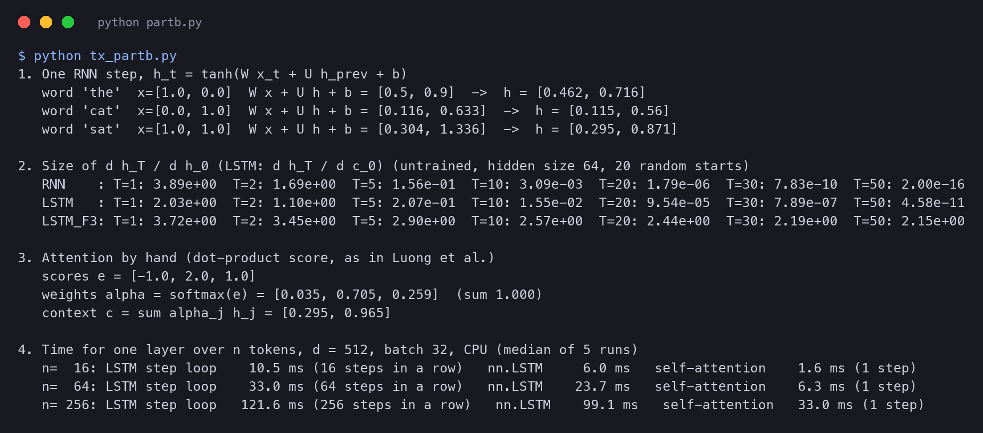
Terminal output of tx_partb.py: one RNN step by hand, the size of the gradient over 1 to 50 steps for a tanh RNN and two LSTMs, the attention example by hand, and the time of an LSTM and a self-attention layer for 16, 64 and 256 tokens — The full output of tx_partb.py, as it ran for this article.

For 256 tokens, the LSTM step loop took 121.6 ms, the built-in nn.LSTM took 99.1 ms, and the self-attention layer took 33.0 ms. Both times grow with $n$ . But the LSTM grows because it needs more steps in a row, and no extra hardware can help with that. Self-attention grows because it does more work in each step, and more hardware does help. On a graphics card, the gap is much larger than on our CPU.

What this run cannot show: these are untrained layers, with no decoder and no training step, on a CPU. It measures one forward pass only. It does not reproduce any number from the papers. Part 4 does the full count of operations and steps that the Transformer paper gives in its Table 1.

From the paperGehring et al. (2017), ConvS2SAbstract

What it says

"Compared to recurrent models, computations over all elements can be fully parallelized during training", and "the number of non-linearities is fixed and independent of the input length".

What it means

In May 2017, one month before the Transformer, a team at Facebook removed the recurrence. Their model uses convolutions: each layer looks at a small window of neighbour tokens, for example 3 words. All windows of a layer can be computed at the same time, so training is fast. They kept Bahdanau-style attention between the encoder and the decoder.

The second phrase is about the vanishing gradient. In an RNN, the path from the first word to the last word passes through $n$ steps, so it gets longer with the sentence. In ConvS2S, the path has a fixed number of layers. But there is a cost: a window of 3 words means that two words far apart need many layers to meet. The Transformer's answer is to let every word look at every other word in one layer.

What the Transformer keeps, and what it drops

Now you can read the Transformer paper as an answer. It keeps the encoder and decoder of sequence to sequence, and the next-word loss of the decoder. It keeps attention from the 2015 paper, with the dot-product score that Luong's paper tested. And it keeps the goal of ConvS2S: all positions at once in training.

It drops the recurrence completely. There is no $h_{t-1}$ in any equation. Inside one sentence, words find each other with attention too. Each word of the input attends to the other words of the input, and this is self-attention.

The title says it directly: attention is all you need. Part 1 starts there.

Key takeaways

An RNN reads one token at a time: $h_t = \tanh(W x_t + U h_{t-1} + b)$ . Step $t$ must wait for step $t-1$ , so the words of a sentence cannot be processed in parallel.
A plain RNN forgets. The learning signal is multiplied once for each step. In our untrained tanh RNN it fell from about 4 to $2 \times 10^{-16}$ over 50 steps.
An LSTM adds a cell and gates. Along the cell, the signal is multiplied only by the forget gate. With the gate near 0.95, our signal stayed near 2 for 50 steps.
Sequence to sequence (2014) used one LSTM to read and one to write. The whole source sentence had to fit into one vector of a fixed size, and long sentences suffered.
Attention (2015) keeps one vector for each source word and makes a new weighted mix for each output word: score, softmax, weighted sum. In our example, "black" got 70% of the weight for "noir".
The dot-product score (Luong et al., 2015) turns attention into matrix multiplications, which graphics cards do very fast.
Each of these models fits in a few lines of code. Our own RNN cell, LSTM cell and additive attention gave the same numbers as PyTorch's nn.RNNCell, nn.LSTMCell and batched code, with a difference of 0.
The bottleneck is measurable. On our digit-reversing toy, the model without attention got 19.2% of 12-digit lists right, and the model with attention got 97.4%.
Recurrence was the last obstacle. GNMT needed 6 days on 96 GPUs. ConvS2S removed recurrence with convolutions, and the Transformer removed it with attention alone.

All the code of this page is in two scripts. tx_partb.py makes the chart and the timing. tx_partb_scratch.py has the cells, the gradient by hand, attention and the digit model.

Next: Part 1 reads the title, the abstract, the introduction and the background section of the paper.

The paper and the code

Paper (arXiv 1706.03762) · tensor2tensor (original code) · Our code for this series

Earlier papers: Sutskever et al. 2014, Bahdanau et al. 2015, Luong et al. 2015, Wu et al. 2016, Gehring et al. 2017

The Road to the Transformer

The task: a sentence in, a sentence out#

Recurrent networks: read one word at a time#

The RNN cell in code#

Why a plain RNN forgets#

The vanishing gradient in code#

LSTM: a memory with gates#

The LSTM cell in code#

Sequence to sequence: one network reads, one network writes#

Sequence to sequence in code#

The bottleneck: one vector for the whole sentence#

Attention: look back at every word#

Bahdanau's score in code#

The same drop on our digit task#

Dot-product attention#

The price of one step at a time#

What the Transformer keeps, and what it drops#

The paper and the code#

The task: a sentence in, a sentence out

Recurrent networks: read one word at a time

The RNN cell in code

Why a plain RNN forgets

The vanishing gradient in code

LSTM: a memory with gates

The LSTM cell in code

Sequence to sequence: one network reads, one network writes

Sequence to sequence in code

The bottleneck: one vector for the whole sentence

Attention: look back at every word

Bahdanau's score in code

The same drop on our digit task

Dot-product attention

The price of one step at a time

What the Transformer keeps, and what it drops

The paper and the code