Circuits, explained · Part 6 of 7 · Covers Analyzing a Two-Layer Model, Induction Heads (function, how they work, checking the theory), the correction to the composition diagram, Pointer Arithmetic with Positional Embeddings

Induction Heads

How a two-layer model learns to continue a pattern it saw earlier in the text. We find the two heads that do it in a real model, test them on random tokens, and break them on purpose.

A Mathematical Framework for Transformer Circuits. Nelson Elhage, Neel Nanda, Catherine Olsson, Tom Henighan, Nicholas Joseph, Ben Mann, Amanda Askell, Yuntao Bai, Anna Chen, Tom Conerly, Nova DasSarma, Dawn Drain, Deep Ganguli, Zac Hatfield-Dodds, Danny Hernandez, Andy Jones, Jackson Kernion, Liane Lovitt, Kamal Ndousse, Dario Amodei, Tom Brown, Jack Clark, Jared Kaplan, Sam McCandlish, Chris Olah. Transformer Circuits Thread, 2021.

Read "Mrs Brindlewick" once, and you can finish "Mrs Br..." the next time it appears. A two-layer transformer learns to do the same with two attention heads that work as a team. This part takes that team apart, in the paper's order and on a real model.

The paper calls the second head of the team an induction head. It is the best-known result of the paper, and later work found the same kind of head in large models. We use the open two-layer model attn-only-2l from the earlier parts. Each piece below shows the exact lines of the paper, then explains them.

The model we study

The paper's two-layer model has 12 heads per layer and no position vectors in the stream. We cannot get those weights. Our model is the open attn-only-2l: two attention layers, eight heads per layer, and no MLP layers. It has one difference that matters later: it adds a learned position vector to the stream of each token.

plain text

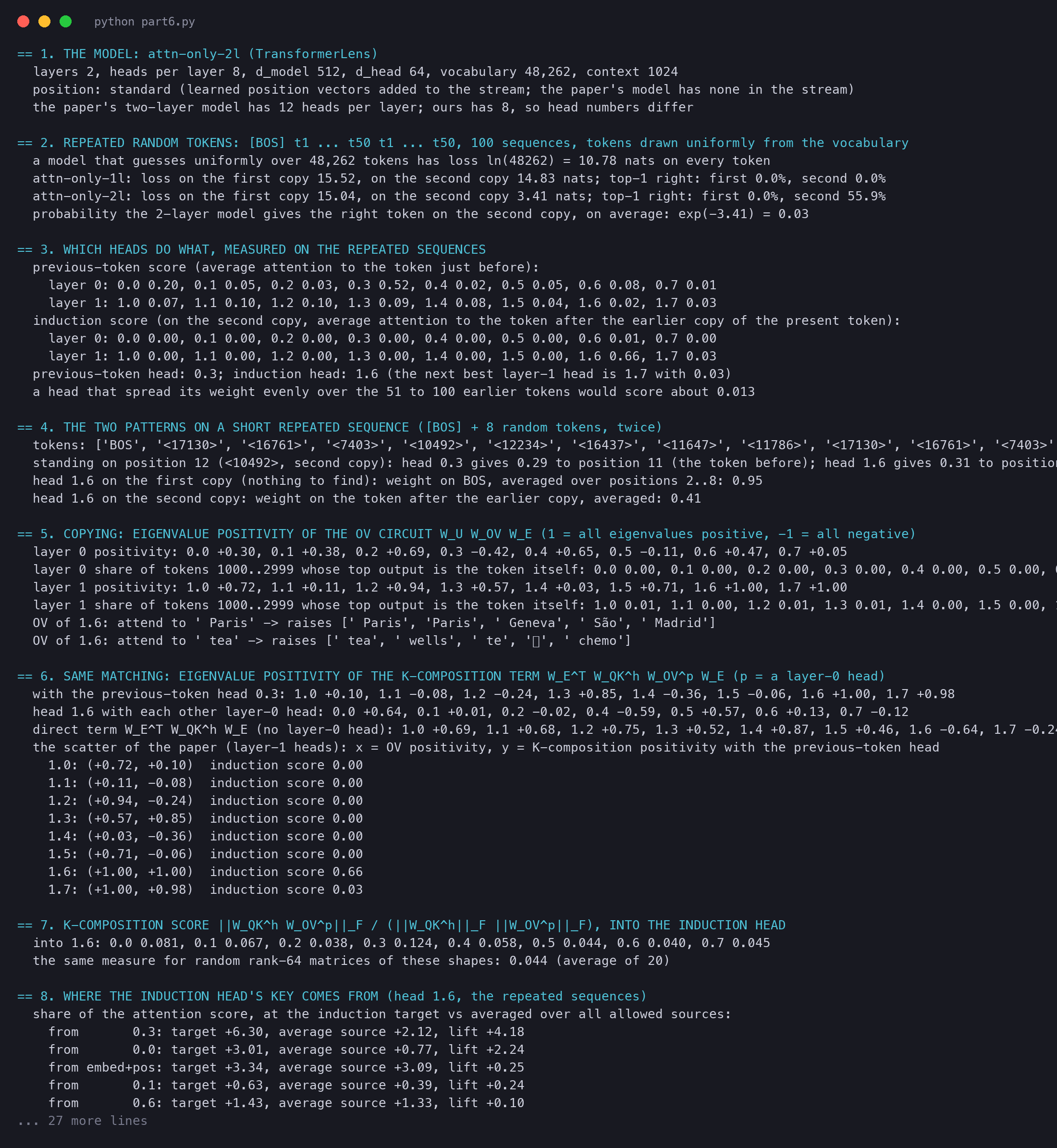
== 1. THE MODEL: attn-only-2l (TransformerLens)
  layers 2, heads per layer 8, d_model 512, d_head 64, vocabulary 48,262, context 1024
  position: standard (learned position vectors added to the stream; the paper's model has none in the stream)
  the paper's two-layer model has 12 heads per layer; ours has 8, so head numbers differ

We name heads as in Part 2: head 0.3 is head 3 of layer 0, and head 1.6 is head 6 of layer 1. Head numbers in our model have no link to the numbers in the paper's model.

A narrow mystery

Part 5 showed three ways in which a layer-1 head can read what a layer-0 head wrote. The paper now looks at one real two-layer model and asks which of those ways it uses.

From the paperAnalyzing a Two-Layer Model

What it says

"Without composition, the model is just a one-layer model with extra heads." In small two-layer models, often "the only type of composition is K-composition between a single first layer head and some of the second layer heads." That first-layer head "primarily attends to the previous token". The second-layer heads "are what we call induction heads".

What it means

A second layer is only useful if it builds on the first one. If the layer-1 heads ignore what the layer-0 heads wrote, then each of them reads only token embeddings. The model is then sixteen independent heads, which is a one-layer model with more heads.

The paper reports that its model uses almost none of the possible connections. One layer-0 head feeds the keys of a few layer-1 heads, and that is all. That is K-composition, the second of the three kinds from Part 5.

So the mystery is small. Most of the model is skip-trigrams, which Part 4 explained. Only one connection is new, and the rest of this part explains what it does.

The paper shows the connections as a diagram. Each dot is a head, and a line joins two heads when a layer-1 head reads strongly from a layer-0 head.

We measured the same score on our model, from the previous-token head into the head we will call the induction head. Part 5 defines it. Here it is enough to know that random matrices of the same shapes score 0.044:

plain text

== 7. K-COMPOSITION SCORE ||W_QK^h W_OV^p||_F / (||W_QK^h||_F ||W_OV^p||_F), INTO THE INDUCTION HEAD
  into 1.6: 0.0 0.081, 0.1 0.067, 0.2 0.038, 0.3 0.124, 0.4 0.058, 0.5 0.044, 0.6 0.040, 0.7 0.045
  the same measure for random rank-64 matrices of these shapes: 0.044 (average of 20)

Head 0.3 scores 0.124, almost three times the random level. Head 0.0 is second with 0.081. The other layer-0 heads are near the random level. So our model has the same shape as the paper's: one main layer-0 head feeds the key of head 1.6.

Looking at the patterns

The paper then invites the reader to look at the attention patterns on the first paragraph of a well-known novel. It shows a special kind of pattern there.

From the paperAnalyzing a Two-Layer Model

What it says

The diagram shows the value-weighted attention pattern: "attention weights scaled by the norm of the value vector at the source position". Heads often use some tokens as "a kind of default or resting position" when nothing matches. The value vectors there are small, so the value-weighted pattern is more informative.

What it means

In Part 2 a head had to spend all its weight, because each row of the pattern adds up to 1. When nothing is worth reading, the weight must go somewhere. Many heads park it on the first token.

A plain pattern then shows a bright column on the first token, and that column hides the real work. If the value vector there is tiny, almost nothing moves. Multiply each weight by the size of its value vector, and the parking spot fades. What is left shows "how big a vector is moved from each position".

What an induction head does

From the paperFunction of Induction Heads

What it says

"Induction heads search over the context for previous examples of the present token." If they find none, "they attend to the first token" and do nothing. If they find one, they look at the next token "and copy it". So they can repeat earlier sequences, "both exactly and approximately".

What it means

Think of reading a story aloud. You reach the word "Mrs" and wonder what comes next. You look back for the last "Mrs", see that "Brindlewick" came after it, and guess "Brindlewick" again.

That is the whole rule, in two steps. Step one: find an earlier copy of the present token. Step two: read the token after that copy, and predict it. The first token is the parking spot from the last box. When there is no earlier copy, the head parks there and adds almost nothing.

The two heads of an induction circuit on a made-up name. In layer 0, a previous-token head gives each position a note that says which token came before it; the position of "indle" gets the note "Br". In layer 1, the induction head stands on the second "Br". Its query looks for the note "Br", finds it at "indle", attends there, and copies "indle" as the prediction.

Why this beats a copying head

From the paperFunction of Induction Heads

What it says

A one-layer copying head does [b] … [a] → [b]. An induction head does [a][b] … [a] → [b]. The two-layer algorithm "knows how the token was previously used and looks out for similar cases". It is also "less vulnerable to distributional shift", because it does not depend on learned statistics about which tokens follow which.

What it means

Read the one-layer pattern slowly. The head stands on [a], sees [b] somewhere earlier, and raises [b]. It needs the weights to know that [b] can follow [a]. Part 4 called this a skip-trigram, and its bugs came from the same place.

The induction pattern needs no such knowledge. It uses only one fact from the text itself: [b] followed [a] before. It would work for two tokens that never met in training.

That is what "less vulnerable to distributional shift" means. Distributional shift is text unlike the training text, such as new names or random strings. Statistics learned in training say nothing about such text, but the rule "repeat what came before" still works.

Our sentence with a made-up name shows the difference. The tokenizer splits " Brindlewick" into " Br", "indle" and "wick". We gave both models the text "The new teacher was Mrs Brindlewick. On Monday the class met Mrs Brindlewick", and looked at the second copy of the name:

plain text

== 10. A MADE-UP NAME IN A SENTENCE
  attn-only-1l: at ' Mrs' (pos 15) the next token ' Br' gets probability 0.01
  attn-only-1l: at ' Br' (pos 16) the next token 'indle' gets probability 0.82
  attn-only-1l: at 'indle' (pos 17) the next token 'wick' gets probability 0.00
  attn-only-2l: at ' Mrs' (pos 15) the next token ' Br' gets probability 0.63; head 1.6 reads '<|BOS|>' (pos 0) with 0.55, adds +4.84 to the logit of ' Br'
  attn-only-2l: at ' Br' (pos 16) the next token 'indle' gets probability 0.93; head 1.6 reads 'indle' (pos 7) with 0.93, adds +11.95 to the logit of 'indle'
  attn-only-2l: at 'indle' (pos 17) the next token 'wick' gets probability 0.98; head 1.6 reads 'wick' (pos 8) with 0.75, adds +13.82 to the logit of 'wick'

The two-layer model gets all three pieces: 0.63, 0.93 and 0.98. On "indle", head 1.6 reads the earlier "wick" with weight 0.75 and adds +13.82 to the logit of "wick". That is the rule from the paper, exactly.

The one-layer model gets "indle" right (0.82), which is a skip-trigram at work: "indle" appeared earlier, so a copying head raised it. But it gives "wick" a probability of 0.00. Its copying heads cannot tell which earlier token is the one to repeat.

The first row of the two-layer model is less clean. On " Mrs", head 1.6's largest single weight (0.55) is on the first token, its parking spot. Yet it still adds +4.84 to " Br". Our log does not show where the rest of its weight went, so we only report what it shows.

The paper's examples

From the paperFunction of Induction Heads

What it says

The strips show the raw attention (red) and the logit effect (blue) of induction head 1:8 on the novel's first paragraph. At a later "D" of "Dursley", the head attends to "urs" after an earlier "D" and raises "urs". At "Pot" of "Potters", it attends to "ters" and raises "ters".

What it means

Each row of a strip is one present token, framed in a box. Red marks where the head looks, and blue marks what it pushes up. In the good rows the red and the blue sit on the same token. The head reads the token after the earlier copy, and predicts that token.

The "logit effect" is the head's output read through the unembedding, as in Part 2. It is the same number our log prints as "adds +13.82 to the logit of 'wick'". Note also the rows where the red sits on the first token: there was nothing to repeat, so the head parked.

The hardest test: random tokens

Text from a novel has a weakness as evidence. A name like "Dursley" is also a common pattern in training text, so other heads may help. The paper removes that help.

From the paperFunction of Induction Heads

What it says

The value-weighted patterns on a random sequence, repeated three times. Head 0:7 is the previous-token head (red), and heads such as 1:8 are induction heads (teal). The pattern shows straight stripes below the diagonal.

What it means

Each stripe is a fixed distance below the diagonal. The string is 20 tokens long, so the token after an earlier copy is always 19 places back. A stripe 19 places below the diagonal means "every token reads the token 19 places back". In the third copy a token can also reach the first copy, 39 places back, which makes a second stripe.

A stripe is the picture of the rule. A head that reads by meaning would make scattered dots. A head that reads by "the token after my last copy" makes a perfect line, because the distance is the same for every token.

Our run

We built 100 sequences. Each is the first token, then 50 random tokens, then the same 50 tokens again. We measure the loss of each model on each copy.

The loss of one token is

\ell=-\ln p_{\text{right}}

Here $p_{\text{right}}$ is the probability the model gave to the token that really came next. Take three small cases by hand. If $p=0.5$ , the loss is $\ln 2\approx0.69$ . If $p=0.05$ , it is about 3.0. A model that guesses evenly over our 48,262 tokens gives each one $p=1/48{,}262$ , so its loss is $\ln 48{,}262\approx10.78$ .

python

logits = model(toks)                                        # toks: [100, 101] = BOS + 50 random + the same 50
loss = -logits.log_softmax(-1)[:, :-1].gather(-1, toks[:, 1:, None])[..., 0]
first, second = loss[:, 1:50].mean(), loss[:, 51:].mean()    # first copy, second copy

plain text

== 2. REPEATED RANDOM TOKENS: [BOS] t1 ... t50 t1 ... t50, 100 sequences, tokens drawn uniformly from the vocabulary
  a model that guesses uniformly over 48,262 tokens has loss ln(48262) = 10.78 nats on every token
  attn-only-1l: loss on the first copy 15.52, on the second copy 14.83 nats; top-1 right: first 0.0%, second 0.0%
  attn-only-2l: loss on the first copy 15.04, on the second copy 3.41 nats; top-1 right: first 0.0%, second 55.9%
  probability the 2-layer model gives the right token on the second copy, on average: exp(-3.41) = 0.03

On the first copy both models do worse than an even guess: about 15 nats against 10.78. They are sure of next tokens that real text would have, and random text punishes that. On the second copy the one-layer model barely moves, from 15.52 to 14.83. The two-layer model drops to 3.41 nats, and its top guess is right 55.9% of the time.

Read 3.41 back as a probability: $e^{-3.41}\approx0.03$ . That number is an average of logarithms, so it is pulled down by the hard tokens. More than half of the tokens are the top guess, which shows that most predictions are much better than 0.03.

Loss at each position, averaged over 100 sequences. The one-layer model stays near 15 nats on both copies. The two-layer model falls from about 15 to about 3 nats right where the second copy starts, at position 51.

The drop is sharp and happens at once. The model does not slowly get used to the string. One token into the repeat, it can already use the rule. A one-layer model cannot, which matches the paper's claim that induction heads need two layers.

Finding the two heads

Which heads do this? We give every head two scores on the repeated sequences. The previous-token score is the average weight a head puts on the position just before. The induction score is the average weight, on the second copy, on the token right after the earlier copy of the present token.

plain text

== 3. WHICH HEADS DO WHAT, MEASURED ON THE REPEATED SEQUENCES
  previous-token score (average attention to the token just before):
    layer 0: 0.0 0.20, 0.1 0.05, 0.2 0.03, 0.3 0.52, 0.4 0.02, 0.5 0.05, 0.6 0.08, 0.7 0.01
    layer 1: 1.0 0.07, 1.1 0.10, 1.2 0.10, 1.3 0.09, 1.4 0.08, 1.5 0.04, 1.6 0.02, 1.7 0.03
  induction score (on the second copy, average attention to the token after the earlier copy of the present token):
    layer 0: 0.0 0.00, 0.1 0.00, 0.2 0.00, 0.3 0.00, 0.4 0.00, 0.5 0.00, 0.6 0.01, 0.7 0.00
    layer 1: 1.0 0.00, 1.1 0.00, 1.2 0.00, 1.3 0.00, 1.4 0.00, 1.5 0.00, 1.6 0.66, 1.7 0.03
  previous-token head: 0.3; induction head: 1.6 (the next best layer-1 head is 1.7 with 0.03)
  a head that spread its weight evenly over the 51 to 100 earlier tokens would score about 0.013

The answer is clear. Head 0.3 puts 0.52 of its weight on the previous token, and head 0.0 is a weaker second with 0.20. Head 1.6 puts 0.66 of its weight on the exact right source, out of 51 to 100 choices. An even spread would score about 0.013, so 0.66 is about fifty times more. No layer-0 head scores above 0.01, which is expected: one layer cannot do this.

This is the same pair as the composition scores showed: head 0.3 feeds head 1.6. Here is what the two patterns look like on a short string of 8 random tokens, repeated:

Two attention patterns on BOS and 8 random tokens t1 to t8, repeated. Head 0.3 (left) puts weight just left of the diagonal, on the previous token. Head 1.6 (right) puts nearly all weight on BOS during the first copy, and a stripe of weight seven places back during the second copy: on the token after the earlier copy.

plain text

  head 1.6 on the first copy (nothing to find): weight on BOS, averaged over positions 2..8: 0.95
  head 1.6 on the second copy: weight on the token after the earlier copy, averaged: 0.41

During the first copy head 1.6 parks 0.95 of its weight on the first token, as the paper said. During the second copy it moves to the stripe. On this short string the stripe holds 0.41 on average, less than the 0.66 of the long strings. Both are far above the even spread.

How the two heads work together

We now know what head 1.6 does. The question is how a head can find "the token after an earlier copy". A head only scores pairs of positions with its query and key. Neither of them, alone, knows about the next token.

From the paperHow Induction Heads Work

What it says

"The central trick to induction heads is that the key is computed from tokens shifted one token back." The query searches for similar keys. "But because keys are shifted", it "finds the next token".

What it means

Picture a coat check where each hook carries the ticket of the coat to its left. You hold ticket 7 and look for the hook that says "7". You find it, but the coat on that hook is the one to the right of coat 7. The tickets are shifted by one place, so a plain search finds the next coat.

In the model, the previous-token head does the shifting. It writes "the token before me" into each position. The induction head's key then reads that note instead of the token itself. So a search for "a key that matches my token" lands one place after the earlier copy.

From the paperHow Induction Heads Work

What it says

The diagram, from a larger model, shows the parts on "Potters" and "Dursley". The key (green) at the source "ters" comes from the token before it, "Pot". The query (teal) is the present token "Pot". They match, so attention (red) moves information from "ters", and the logit effect (purple) raises "ters".

What it means

Follow the colours from bottom to top. Green: the key of "ters" carries "Pot", because the previous-token head copied it there. Teal: the query of the present "Pot" asks for "Pot". The two meet, and the red line carries "ters" up to the present position.

The last step is the OV circuit from Part 2. The head reads "ters" and copies it, so "ters" goes up as the next token. The QK side finds the place; the OV side copies the token. These are the two separate jobs of any head, now chained across two layers.

The K-composition term, step by step

The paper writes the trick as a term of the QK circuit. We build it from the pieces of Part 2 and Part 5. Leave out positions and layer norm for now, as the paper does.

The stream at a source position $j$ , as layer 1 reads it, holds the token's embedding plus what layer 0 wrote. Keep only the previous-token head $p$ , and say that it reads the position just before with weight 1:

x_j=W_{\mathrm{E}}\,t_j+W_{\mathrm{OV}}^{p}\,W_{\mathrm{E}}\,t_{j-1}

Read it left to right. $t_j$ is the one-hot vector of the token at $j$ , and $W_{\mathrm{E}}t_j$ is its embedding. The second term is head $p$ 's output: the embedding of the token before $j$ , passed through its OV matrix. The destination $i$ has only its own embedding, $x_i=W_{\mathrm{E}}t_i$ , in this simple view.

The attention score of the layer-1 head $h$ is $s_{ij}=x_i^\top W_{\mathrm{QK}}^{h}\,x_j$ . Put the two streams in and multiply out:

\begin{aligned} s_{ij}={}&t_i^\top\big({W_{\mathrm{E}}}^{\top}W_{\mathrm{QK}}^{h}W_{\mathrm{E}}\big)\,t_j\\ &+t_i^\top\big({W_{\mathrm{E}}}^{\top}W_{\mathrm{QK}}^{h}W_{\mathrm{OV}}^{p}W_{\mathrm{E}}\big)\,t_{j-1} \end{aligned}

The first line is the plain QK circuit of Part 2: present token against source token. The second line is new. It compares the present token $t_i$ with the token before the source, $t_{j-1}$ . Call its matrix $W$ :

W={W_{\mathrm{E}}}^{\top}W_{\mathrm{QK}}^{h}W_{\mathrm{OV}}^{p}W_{\mathrm{E}}

$W$ is a token-by-token table, like the circuits of Part 2. Its entry in row $a$ , column $b$ says how much a destination token $a$ likes a source whose previous token is $b$ . Now suppose $W$ is large on its diagonal and small elsewhere. Then the score is large exactly when $t_{j-1}=t_i$ : the token before the source equals the present token. That is the induction rule, written as a matrix.

From the paperHow Induction Heads Work

$The paragraph on the minimal way to create an induction head: K-composition with a previous token head shifts the key forward one token, creating a term Id ⊗ A^{h-1} ⊗ W in the QK circuit; if W matches cases where the tokens are the same, the QK version of a copying matrix, the term raises attention when the previous token before the source equals the destination token$

What it says

"The minimal way to create an induction head" is K-composition with a previous-token head. It creates a term $\text{Id}\otimes A^{h_{-1}}\otimes W$ in the QK circuit, where $A^{h_{-1}}$ attends to the previous token. Suppose $W$ matches equal tokens, like "the QK version of a" copying matrix. Then the term raises attention "when the previous token before the source position is the same as the destination token".

What it means

This is our derivation in the paper's notation. The middle factor $A^{h_{-1}}$ is the shift: it moves each source back by one token. The right factor $W$ is the table we just built. "Same matching" means $W$ behaves like the identity: token $a$ matches token $a$ .

The bracket notes that other models build longer shifts, $A^{h_{-1}}\otimes A^{h_{-2}}\otimes W$ , by using a head that looks a bit further back. Then a head can match two tokens before the source, not one. We see a hint of this in our model: head 0.0, which also looks back but less sharply, feeds head 1.6 too.

A tiny example by hand. Our toy script builds the whole circuit with three tokens, a, b and c. The stream has six numbers. Three say "this token is a, b or c". Three say "the token before me was a, b or c". The sequence is a b c a. We want the last "a" to predict "b".

Layer 0 is a previous-token head. It copies each token's "this token" numbers into the "token before" numbers of the next position. Layer 1 is the induction head, with $W_{\mathrm{QK}}$ that multiplies "this token" at the destination with "token before" at the source, times 4:

plain text

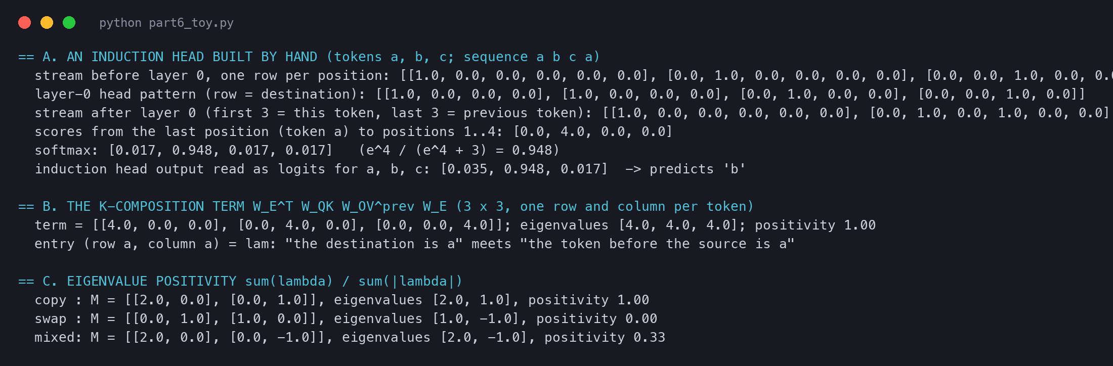
== A. AN INDUCTION HEAD BUILT BY HAND (tokens a, b, c; sequence a b c a)
  stream after layer 0 (first 3 = this token, last 3 = previous token): [[1.0, 0.0, 0.0, 0.0, 0.0, 0.0], [0.0, 1.0, 0.0, 1.0, 0.0, 0.0], [0.0, 0.0, 1.0, 0.0, 1.0, 0.0], [1.0, 0.0, 0.0, 0.0, 0.0, 1.0]]
  scores from the last position (token a) to positions 1..4: [0.0, 4.0, 0.0, 0.0]
  softmax: [0.017, 0.948, 0.017, 0.017]   (e^4 / (e^4 + 3) = 0.948)
  induction head output read as logits for a, b, c: [0.035, 0.948, 0.017]  -> predicts 'b'

Check it by hand. Position 2 holds "b", with the note "the token before me was a", and the last position holds "a". Only position 2 has a note that matches "a", so only it scores 4. The softmax gives it $e^4/(e^4+3)\approx0.948$ . The head's OV circuit copies what is at position 2, which is "b". So "b" gets 0.948, the largest logit.

The $W$ table of this toy is $4$ times the identity, a pure "same matching" table:

plain text

== B. THE K-COMPOSITION TERM W_E^T W_QK W_OV^prev W_E (3 x 3, one row and column per token)
  term = [[4.0, 0.0, 0.0], [0.0, 4.0, 0.0], [0.0, 0.0, 4.0]]; eigenvalues [4.0, 4.0, 4.0]; positivity 1.00

Where the real key comes from

Does head 1.6 really get its match from head 0.3? We can check it on the real model, with positions, biases and layer norm included. The stream that layer 1 reads is a sum: embedding plus position, plus each layer-0 head's output, plus a bias. Layer norm only divides the sum by one number per position. So the key, and the score, also split into one part per piece.

python

parts = {'embed+pos': cache['hook_embed'] + cache['hook_pos_embed']}
for p in range(8):
    parts[f'0.{p}'] = cache['blocks.0.attn.hook_z'][:, :, p] @ model.W_O[0, p]   # what head 0.p wrote
keys = {k: (centre(v) / scale) @ model.W_K[1, 6] for k, v in parts.items()}       # the key, one part at a time

For each part we compare its share of the score at the right source with its share at an average allowed source. The difference is the lift: how much that part helps the right source win.

plain text

== 8. WHERE THE INDUCTION HEAD'S KEY COMES FROM (head 1.6, the repeated sequences)
  share of the attention score, at the induction target vs averaged over all allowed sources:
    from       0.3: target +6.30, average source +2.12, lift +4.18
    from       0.0: target +3.01, average source +0.77, lift +2.24
    from embed+pos: target +3.34, average source +3.09, lift +0.25
    from       0.1: target +0.63, average source +0.39, lift +0.24
    from       0.6: target +1.43, average source +1.33, lift +0.10
    from       0.2: target +1.23, average source +1.16, lift +0.07
    from       0.5: target -0.94, average source -0.96, lift +0.02
    from      bias: target +9.76, average source +9.78, lift -0.02
    from       0.4: target +1.41, average source +1.41, lift +0.00
    from       0.7: target -0.74, average source -0.75, lift +0.00
    key bias part: +5.49 (the same for every source, so the softmax ignores it)
  sum of the parts at the target 30.93; the model's own score 30.93

How much each part of the stream lifts head 1.6's score at the right source, above an average source. Head 0.3 gives +4.18 and head 0.0 gives +2.24. The token and position embeddings give only +0.25, and every other layer-0 head gives less than 0.3.

The parts add up to the model's own score, 30.93, so the split is exact. Almost all of the lift comes from what heads 0.3 and 0.0 wrote: +4.18 and +2.24. The source token's own embedding gives only +0.25. So head 1.6 does not choose its source by what the source is. It chooses it by the note that the previous-token heads left there. That is K-composition, measured.

Checking the theory from the weights

The tests so far ran the model on text. The paper also checks the theory from the weights alone, with no text at all.

The statistic is

\text{positivity}(M)=\frac{\sum_k \lambda_k}{\sum_k \lvert\lambda_k\rvert}

The top sums the eigenvalues $\lambda_k$ of $M$ , and the bottom sums their sizes. If every eigenvalue is positive, top and bottom are equal and the score is 1. If every eigenvalue is negative, the score is $-1$ . A copying matrix sends each token back toward itself, so its eigenvalues are mostly positive and its score is near 1.

Three 2 × 2 matrices show the range:

plain text

== C. EIGENVALUE POSITIVITY sum(lambda) / sum(|lambda|)
  copy : M = [[2.0, 0.0], [0.0, 1.0]], eigenvalues [2.0, 1.0], positivity 1.00
  swap : M = [[0.0, 1.0], [1.0, 0.0]], eigenvalues [1.0, -1.0], positivity 0.00
  mixed: M = [[2.0, 0.0], [0.0, -1.0]], eigenvalues [2.0, -1.0], positivity 0.33

The "copy" matrix keeps each token, so it scores 1. The "swap" matrix turns a into b and b into a, so it copies nothing and scores 0. The "mixed" one keeps one token and flips the other: $(2-1)/(2+1)=0.33$ .

The real tables are 48,262 × 48,262, too big for eigenvalues. But a product $AB$ and the product in the other order, $BA$ , have the same non-zero eigenvalues. So the eigenvalues of $W_{\mathrm{U}}W_{\mathrm{OV}}W_{\mathrm{E}}$ are those of the 512 × 512 matrix $W_{\mathrm{OV}}W_{\mathrm{E}}W_{\mathrm{U}}$ . The same trick works for the K-composition term.

plain text

== 5. COPYING: EIGENVALUE POSITIVITY OF THE OV CIRCUIT W_U W_OV W_E (1 = all eigenvalues positive, -1 = all negative)
  layer 1 positivity: 1.0 +0.72, 1.1 +0.11, 1.2 +0.94, 1.3 +0.57, 1.4 +0.03, 1.5 +0.71, 1.6 +1.00, 1.7 +1.00
  layer 1 share of tokens 1000..2999 whose top output is the token itself: 1.0 0.01, 1.1 0.00, 1.2 0.01, 1.3 0.01, 1.4 0.00, 1.5 0.00, 1.6 0.99, 1.7 0.26
  OV of 1.6: attend to ' Paris' -> raises [' Paris', 'Paris', ' Geneva', ' São', ' Madrid']

== 6. SAME MATCHING: EIGENVALUE POSITIVITY OF THE K-COMPOSITION TERM W_E^T W_QK^h W_OV^p W_E (p = a layer-0 head)
  with the previous-token head 0.3: 1.0 +0.10, 1.1 -0.08, 1.2 -0.24, 1.3 +0.85, 1.4 -0.36, 1.5 -0.06, 1.6 +1.00, 1.7 +0.98

Head 1.6 scores +1.00 on both. Its OV circuit is a near-perfect copier: for 99% of tokens 1,000 to 2,999, the top output is the token itself. Its K-composition table with head 0.3 is a near-perfect matcher. These two numbers come from the weights only, with no text.

From the paperChecking the Mechanistic Theory

What it says

Each second-layer head is a point. Across is the eigenvalue positivity of its OV circuit $W_{\mathrm{U}}W_{\mathrm{OV}}^{h}W_{\mathrm{E}}$ . Up is the positivity of $W$ in the K-composition term, ${W_{\mathrm{E}}}^{\top}W_{\mathrm{QK}}^{h}W_{\mathrm{OV}}^{h_{-1}}W_{\mathrm{E}}$ . "All the induction heads are at the extreme of OV and QK positivity."

What it means

A head in the top right corner both matches and copies. That is the full recipe of an induction head, read straight from the weights. The other heads are scattered, because they do other jobs.

The inset zooms into the corner, because the induction heads sit very close to the point (1, 1). They are not just positive: they are almost perfectly positive.

Here is the same plot for our model:

The eight layer-1 heads of attn-only-2l. Across: OV circuit positivity. Up: positivity of the K-composition term with head 0.3. Heads 1.6 and 1.7 sit in the top right corner, near (1, 1). The other six heads are spread out.

Two heads land in the corner: 1.6, and 1.7 at (+1.00, +0.98). Head 1.7 is a surprise, because its induction score on our sequences was only 0.03. Its weights have the recipe, but on this data it rarely acts on it. When we remove it (next section), the loss on the second copy rises from 3.41 to 3.77, so it helps a little. These numbers do not say why it attends so weakly. Its plain QK circuit, the first line of our derivation, may pull against the match.

From the paperChecking the Mechanistic Theory

What it says

"One might wonder if this observation is circular." The heads were picked because of large K-composition. But the K-composition matrix is "extremely biased towards positive eigenvalues", and nothing forced that. Nor did anything force the OV circuits to be positive.

What it means

A fair worry: if you pick heads by one property and then measure the same property, of course you find it. The paper answers that the two measures are different. The composition score asks "how much does this head read from that one?" The positivity asks "does it read in a matching way?"

A strong connection could have been strongly negative, an "avoid the same token" table. It could have been a mix. It came out almost purely positive, which is what the induction story predicts and nothing else does. The OV side was not used to pick the heads at all.

Our run adds a control. The same positivity for head 1.6, but with the other layer-0 heads in place of 0.3:

plain text

  head 1.6 with each other layer-0 head: 0.0 +0.64, 0.1 +0.01, 0.2 -0.02, 0.4 -0.59, 0.5 +0.57, 0.6 +0.13, 0.7 -0.12
  direct term W_E^T W_QK^h W_E (no layer-0 head): 1.0 +0.69, 1.1 +0.68, 1.2 +0.75, 1.3 +0.52, 1.4 +0.87, 1.5 +0.46, 1.6 -0.64, 1.7 -0.24

With other heads the score falls to between -0.59 and +0.64. The next best is head 0.0, the second previous-token head. And head 1.6's direct term, present token against source token, is negative (-0.64). On its own, head 1.6 slightly avoids a source that equals the present token. It only matches through the shifted note.

Breaking the circuit on purpose

The weights tell a clean story. A last test is to remove a part and see what breaks. This is our own test; the paper's term-importance section, in Part 5, uses a related idea.

python

mean = cache['blocks.0.attn.hook_z'][:, :, 3].mean((0, 1))    # head 0.3's average result vector
def hook(z, hook):
    z[:, :, 3] = mean                                         # same vector at every position
    return z
logits = model.run_with_hooks(toks, fwd_hooks=[('blocks.0.attn.hook_z', hook)])

plain text

== 9. ABLATIONS: REPLACE ONE HEAD'S RESULT VECTORS WITH THEIR AVERAGE OVER ALL POSITIONS AND SEQUENCES
  no ablation:            loss first 15.04, second 3.41; induction score of 1.6 0.66
  ablate 0.3 (the previous-token head): loss first 13.68, second 11.85; induction score of 1.6 0.06
  ablate 0.0 (the second most previous-token head): loss first 14.27, second 6.33; induction score of 1.6 0.37
  ablate 0.7 (the least previous-token layer-0 head): loss first 17.97, second 4.15; induction score of 1.6 0.64
  ablate 1.6 (the induction head): loss first 14.25, second 13.04; induction score of 1.6 0.66
  ablate 1.7 (the second induction-like head): loss first 15.04, second 3.77; induction score of 1.6 0.66
  ablate 1.1 (the least induction-like layer-1 head): loss first 14.86, second 3.33; induction score of 1.6 0.64

Loss on the second copy after replacing one head with its average output. With no ablation it is 3.41 nats. Replacing head 0.3 raises it to 11.85, and replacing head 1.6 raises it to 13.04. Replacing head 0.0 raises it to 6.33. The other heads change it by less than 0.8.

Remove head 0.3, and head 1.6 loses its way: its induction score falls from 0.66 to 0.06. The loss on the second copy jumps from 3.41 to 11.85. Head 1.6 itself is untouched, yet it no longer finds the right source. The note it searched for is gone.

Remove head 1.6, and its pattern is unchanged (0.66), because nothing before it changed. But its output is gone, and the loss on the second copy rises to 13.04. So the two heads are both needed: one to find the place, one to copy.

The controls behave as expected. Head 0.0 is a partial helper (6.33). Heads 1.7, 1.1 and 0.7 change the second-copy loss by less than 0.8. Head 0.7 has one odd effect: the first-copy loss rises to 17.97. That copy is random text, so the change says little about induction, and we do not explain it here.

What these tests cannot show: mean ablation is only one way to remove a head. Other ways, such as setting it to zero, can give different numbers. And random tokens are not real text. They isolate induction, but they say nothing about how much the model uses it on ordinary prose.

The correction to the diagram

After publication, the authors found a bug that changed one diagram: the composition diagram at the start of this part.

From the paperCorrection: Attention Head Composition Diagram

What it says

A library bug changed the order of a matrix product inside the composition score. It measured "the extent to which the induction head's query is built from the same subspace that the previous token head moved data into". So it responded very strongly to induction composition and filtered out other kinds.

What it means

Some quantities do not care about the order of a product, such as the trace and the eigenvalues; we used that fact above. The Frobenius norm of the composition score does care. The library swapped the order anyway, so it computed a different number.

By luck, the wrong number is a fine detector of induction. It asks whether the query reads the same subspace that the previous-token head writes to, which is the recipe of this part. So the old diagram showed the induction circuit very clearly, and hid most other composition.

From the paperCorrection: Attention Head Composition Diagram

What it says

"the importance of K-composition with the previous token head remains unchanged". The main addition is that "two of the induction heads also rely on a head which attends to the last several tokens".

What it means

This matches the bracket in the How Induction Heads Work section: real induction heads often use more than the minimal circuit. A head that looks at the last several tokens gives a wider note, such as "the two tokens before me". Matching on more context makes fewer false matches.

Our model shows the same pattern. Head 0.0 is a weaker, wider previous-token head (score 0.20). It has the second-largest composition score into head 1.6 (0.081) and the second-largest lift (+2.24). Removing it raised the second-copy loss to 6.33. Our measures used the corrected order of the product.

What attention patterns hide

Induction heads also teach a lesson about reading attention patterns. The paper makes it in its related-work section.

From the paperCriticism of Attention as Explanation

What it says

Attention patterns can "both be very informative and also misleading". The induction head's own pattern is informative. But the head is "totally reliant on a previous token head in the prior layer" to decide where to attend. Gradient-based attribution may miss this too, because "its softmax will be saturated".

What it means

Look only at head 1.6's pattern, and you would say "it reads the earlier wick, and predicts wick". That is true, and useful. But it hides the reason it chose that position: a note written by a different head, one layer down.

Look only at head 0.3's pattern, and you would say "it reads the previous token; how dull". You would miss that this dull head is half of the most important circuit in the model. Our ablation showed it: removing it raised the loss on the second copy from 3.41 to 11.85.

The last sentence is about another tool. A saturated softmax gives nearly all its weight to one source, so small changes to the key barely move it. A method that measures importance by such small changes then says the key does not matter, which is wrong.

Another way to build one

The paper's appendix notes that the K-composition circuit is not the only way to build an induction head. Our model has position vectors in its stream, so this note applies to it.

From the paperPointer Arithmetic with Positional Embeddings

What it says

Transformers can do "pointer arithmetic" on position vectors. In GPT-2, "an induction head was implemented using this approach". One head attends to an earlier copy of the token and returns its position. Then another head's query, built by Q-composition, is made by "rotating the positional embedding forward one token".

What it means

Think of looking up a word in a book's index. The first head finds the page where the word appeared and writes down the page number. The second head adds one to that number and turns to the next page.

The result is the same induction rule, built in a different way. Here the first head works on the query side (Q-composition), not on the key side. This needs position vectors in the stream; the paper's own small models have none, so they could only use the key-side trick.

For us it is a warning. Two models can do the same thing with different circuits. A test such as the repeated random tokens finds the behaviour; only the weights show which circuit does it. In our model the weights point to the key side: head 0.3's note gives the largest lift, and removing it breaks the head.

Key takeaways

An induction head completes [A][B] ... [A] → [B]. It finds an earlier copy of the present token, attends to the token after it, and copies that token. It needs two layers.
It is a team of two heads. A layer-0 previous-token head writes "the token before me" into each position. The induction head's key reads that note, so a search for the present token lands one place later. In our model the team is head 0.3 and head 1.6.
Random repeated tokens isolate it. On 100 sequences of 50 random tokens shown twice, attn-only-2l fell from 15.04 to 3.41 nats on the second copy, and got 55.9% of tokens right. attn-only-1l only fell from 15.52 to 14.83.
Head 1.6 puts 0.66 of its weight on the exact right source, out of 51 to 100 choices; an even spread would give about 0.013.
The trick is a K-composition term ${W_{\mathrm{E}}}^{\top}W_{\mathrm{QK}}^{h}W_{\mathrm{OV}}^{p}W_{\mathrm{E}}$ that compares the present token with the token before the source. When it is close to the identity, it is a "same matching" table.
The weights alone confirm it. Head 1.6 has eigenvalue positivity +1.00 for both its OV circuit (copying) and its K-composition term with head 0.3 (matching). Its direct QK term is -0.64.
The note, not the token, picks the source. Of head 1.6's lift at the right source, head 0.3 gives +4.18 and head 0.0 gives +2.24; the source token's own embedding gives +0.25.
Both heads are needed. Mean-ablating head 0.3 cut head 1.6's induction score from 0.66 to 0.06 and raised the second-copy loss to 11.85; mean-ablating head 1.6 raised it to 13.04.
Attention patterns alone mislead. The previous-token head looks dull, but it is half of the circuit. Other models can build the same behaviour another way, for example with pointer arithmetic on position vectors.

Next, in Part 7: what the paper left out, MLP layers above all. Then what came after: induction heads in large models, superposition, dictionary learning and circuit tracing. Part 7 also ties the whole series together.

Run it yourself

The script circuits_part6.py runs every real-model test of this part: the repeated random tokens, the head scores, the eigenvalue positivity, the composition scores, the split of the key and the ablations. circuits_part6_toy.py builds the three-token induction circuit by hand. Both run on the CPU; the first one took a few minutes while other jobs ran on the same machine.

bash

pip install torch "transformer_lens<4"
python circuits_part6.py        # writes results/part6.json and results/part6_stdout.txt
python circuits_part6_toy.py    # writes results/part6_toy.json

Terminal output of circuits_part6.py: the model, the loss on both copies of the repeated random tokens, the previous-token and induction scores of every head, the two patterns on a short sequence, the eigenvalue positivity of the OV circuits and of the K-composition terms, and the composition scores — The first part of the output of circuits_part6.py.

Terminal output of circuits_part6_toy.py: the hand-built induction circuit on the sequence a b c a, its K-composition term, and eigenvalue positivity on three 2 by 2 matrices — The output of circuits_part6_toy.py.

The paper and the code

A Mathematical Framework for Transformer Circuits (2021) · our scripts for this series

Induction Heads

The model we study#

A narrow mystery#

Looking at the patterns#

What an induction head does#

Why this beats a copying head#

The paper's examples#

The hardest test: random tokens#

Our run#

Finding the two heads#

How the two heads work together#

The K-composition term, step by step#

Where the real key comes from#

Checking the theory from the weights#

Breaking the circuit on purpose#

The correction to the diagram#

What attention patterns hide#

Another way to build one#

The paper and the code#

The model we study

A narrow mystery

Looking at the patterns

What an induction head does

Why this beats a copying head

The paper's examples

The hardest test: random tokens

Our run

Finding the two heads

How the two heads work together

The K-composition term, step by step

Where the real key comes from

Checking the theory from the weights

Breaking the circuit on purpose

The correction to the diagram

What attention patterns hide

Another way to build one

The paper and the code