Circuits, explained · Part 5 of 7 · Covers Two-Layer Attention-Only Transformers, Three Kinds of Composition, Path Expansion of Logits and of Attention Scores, Analyzing a Two-Layer Model, Term Importance Analysis, Virtual Attention Heads

Two-Layer Models: How Heads Compose

With a second layer, one head can read what an earlier head wrote. We follow the paper's three kinds of composition, expand the logits and the attention scores into paths, and measure which paths matter in a real two-layer model.

A Mathematical Framework for Transformer Circuits. Nelson Elhage, Neel Nanda, Catherine Olsson, Tom Henighan, Nicholas Joseph, Ben Mann, Amanda Askell, Yuntao Bai, Anna Chen, Tom Conerly, Nova DasSarma, Dawn Drain, Deep Ganguli, Zac Hatfield-Dodds, Danny Hernandez, Andy Jones, Jackson Kernion, Liane Lovitt, Kamal Ndousse, Dario Amodei, Tom Brown, Jack Clark, Jared Kaplan, Sam McCandlish, Chris Olah. Transformer Circuits Thread, 2021.

A one-layer model can only look up tables of token pairs and skip-trigrams. Give it a second layer, and a head can read what another head wrote a moment before. That small change is where the paper's most interesting results begin.

The real model here is attn-only-2l: two layers of attention, eight heads per layer, and nothing else. We run it on 3,072 tokens of ordinary English text from WikiText.

Why depth matters

From the paperTwo-Layer Attention-Only Transformers

What it says

One intuition for the power of deep models is that "depth allows composition". "Composition of attention heads is the key difference between one-layer and two-layer attention-only transformers". Without it, a second layer would only add more heads for skip-trigrams. With it, two-layer models become "much more like a computer program running an algorithm" than look-up tables.

What it means

Think of two clerks at one desk. The first clerk writes notes on a shared board. The second clerk reads the board before doing their own job. The second clerk can now do things that neither clerk could do alone, because the first one prepared the ground.

In a one-layer model, every head reads only the token embeddings. Part 4 showed what that gives: a bigram table and a set of skip-trigrams, such as "keep … in mind". A skip-trigram is a rule of the form "if token A appears earlier and the current token is B, raise C". All of it is a fixed table that you can read from the weights.

In a two-layer model, a head in the second layer reads a stream that the first layer has already changed. So what it sees is no longer a plain token. It can be "the token that came after the word I saw before". Rules about such derived facts are what turn a table into a small algorithm.

Three kinds of composition

Every head reads the stream through three matrices and writes back through one. So there are three places where a later head can pick up an earlier head's work.

From the paperThree Kinds of Composition

What it says

Every head reads subspaces of the residual stream chosen by $W_{\mathrm{Q}}$ , $W_{\mathrm{K}}$ and $W_{\mathrm{V}}$ , and writes to a subspace chosen by $W_{\mathrm{O}}$ . Head vectors are much smaller than the stream: $d_\text{head}/d_\text{model}$ is around 1/10 to 1/100. So "attention heads operate on small subspaces and can easily avoid significant interaction".

What it means

Picture the stream as a wide whiteboard and each head as a person who only reads a narrow strip of it. A strip is narrow, and the board is wide. Two people can work all day on different strips and never see each other's writing.

So composition is not automatic. A later head only composes with an earlier head if its strip overlaps the strip that the earlier head writes. Training decides whether that happens. In our model $d_\text{head}/d_\text{model}=64/512=0.125$ , which is near the top of the paper's range.

From the paperThree Kinds of Composition

What it says

There are three options. In Q-composition, $W_{\mathrm{Q}}$ reads a subspace affected by a previous head. In K-composition, $W_{\mathrm{K}}$ does, and in V-composition, $W_{\mathrm{V}}$ does. Q- and K-composition "both affect the attention pattern". V-composition affects what a head moves, and creates "virtual attention heads". "Composing movement of information with movement of information gives movement of information."

What it means

Recall from Part 2 that a head does two jobs. Its QK circuit decides where to look, and its OV circuit decides what to carry. Q- and K-composition change the "where" job. V-composition changes the "what" job.

Think of a post office. In Q-composition, a note on the parcel changes which address the clerk looks for. In K-composition, a note on each house changes which house matches. In V-composition, the clerk carries a parcel that another clerk already carried once.

The last kind is the simplest. A parcel moved twice is still a moved parcel. Two V-composed heads act like one new head that moves information in one step. Q- and K-composition are richer, because a changed "where" can make attention patterns that no single head could make.

Three kinds of composition. A layer-0 head writes into the stream. A layer-1 head reads the stream through W_Q, W_K and W_V. If its W_Q reads the layer-0 head's output, that is Q-composition; if its W_K does, K-composition; if its W_V does, V-composition.

The logits as a sum of paths

From the paperPath Expansion of Logits

What it says

The most basic question is "how are the logits computed?". As for the one-layer model, the paper writes the model as a product with one factor per layer. Then it expands the product into a sum "where every term is an end-to-end path through the model".

What it means

Think of a river with two weirs. Water can flow straight past both weirs, or it can be diverted at the first, at the second, or at both. Every drop at the sea took one of these four routes. Count the drops on each route, and you know where the water came from.

The model works the same way. Each layer either lets the stream pass or adds a head's output. The path expansion lists every route from the input tokens to the logits, so each route can be studied alone. Part 3 did this for one layer; now there are two.

Here is the paper's whole equation, with its picture of each term:

From the paperPath Expansion of Logits

What it says

The whole model $T$ is a product of four factors: the unembedding, layer 2, layer 1 and the embedding. Each layer is $\text{Id}$ plus the sum of its heads. The product expands into three groups. The "direct path" term contributes to bigram statistics. Then come the "individual attention head" terms, and the "virtual attention head" terms, which "correspond to V-composition".

What it means

Read the top line from right to left, the way the data flows. First the embedding $W_{\mathrm{E}}$ . Then layer 1, where the stream either passes ( $\text{Id}$ ) or goes through one of its heads. Then layer 2, with the same choice. Finally the unembedding $W_{\mathrm{U}}$ .

The bottom line is the same thing multiplied out. Each term is one route. The small diagrams show which boxes each route passes through: no head, one head, or one head in each layer.

The derivation

The expansion is the same algebra as $(1+a)(1+b)=1+a+b+ab$ , with matrices. Write $H_1$ for the heads of the first layer and $H_2$ for the second. From Part 2, one head is $A^h\otimes W_{\mathrm{OV}}^h$ : its attention pattern $A^h$ mixes tokens, and $W_{\mathrm{OV}}^h=W_{\mathrm{O}}^hW_{\mathrm{V}}^h$ acts inside each token. A layer adds its heads to the stream, so a layer is $\text{Id}+\sum_h A^h\otimes W_{\mathrm{OV}}^h$ .

So the whole model is:

\begin{aligned} T={}&(\text{Id}\otimes W_{\mathrm{U}})\\ &\cdot\Big(\text{Id}+\sum_{h\in H_2}A^h\otimes W_{\mathrm{OV}}^h\Big)\\ &\cdot\Big(\text{Id}+\sum_{h\in H_1}A^h\otimes W_{\mathrm{OV}}^h\Big)\\ &\cdot(\text{Id}\otimes W_{\mathrm{E}}) \end{aligned}

Multiply the two middle brackets out. You get four groups: $\text{Id}\cdot\text{Id}$ , layer-2 heads times $\text{Id}$ , $\text{Id}$ times layer-1 heads, and layer-2 heads times layer-1 heads. The mixed-product rule from Part 2, $(A\otimes B)(C\otimes D)=(AC)\otimes(BD)$ , turns each product of two heads into one term:

\begin{aligned} &(A^{h_2}\otimes W_{\mathrm{OV}}^{h_2})(A^{h_1}\otimes W_{\mathrm{OV}}^{h_1})\\ &=(A^{h_2}A^{h_1})\otimes(W_{\mathrm{OV}}^{h_2}W_{\mathrm{OV}}^{h_1}) \end{aligned}

Now attach $\text{Id}\otimes W_{\mathrm{U}}$ on the left and $\text{Id}\otimes W_{\mathrm{E}}$ on the right, and use the same rule once more. The result is the paper's bottom line:

\begin{aligned} T={}&\text{Id}\otimes W_{\mathrm{U}}W_{\mathrm{E}}\\ &+\sum_{h\in H_1\cup H_2}A^h\otimes\big(W_{\mathrm{U}}W_{\mathrm{OV}}^hW_{\mathrm{E}}\big)\\ &+\sum_{h_2\in H_2}\sum_{h_1\in H_1}(A^{h_2}A^{h_1})\\ &\qquad\otimes\big(W_{\mathrm{U}}W_{\mathrm{OV}}^{h_2}W_{\mathrm{OV}}^{h_1}W_{\mathrm{E}}\big) \end{aligned}

Read it group by group. The first line is the direct path: embed a token and unembed it at once, which is the bigram table of Part 1. The second line has one term per head, in either layer, that reads the embeddings directly. These are the same skip-trigram terms as in the one-layer model. The last two lines hold one term for every pair of a layer-2 head and a layer-1 head. In each, the layer-1 head moves information, and then the layer-2 head moves the result again.

A toy example. Take a stream of one number per token and three tokens, $x_0=(1,2,3)$ . Each layer has one head. In layer 1, each token reads the token before it (token 1 reads itself), and the OV "matrix" is the number $w_1=0.5$ . In layer 2, token 2 reads tokens 1 and 2 half each, the others read themselves, and $w_2=2$ .

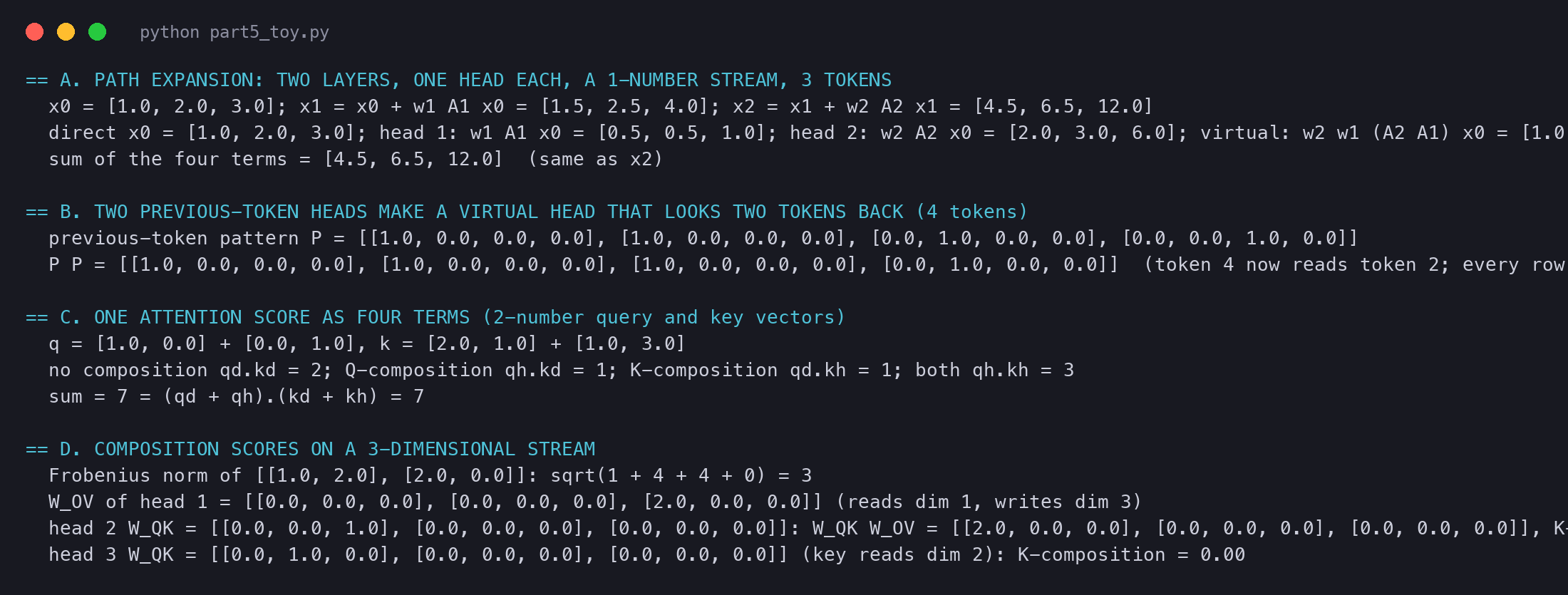
The toy path expansion. The direct path is (1, 2, 3). Head 1 alone adds (0.5, 0.5, 1). Head 2 alone, reading the embeddings, adds (2, 3, 6). The virtual head, head 2 reading what head 1 wrote, adds (1, 1, 2). The four rows add up to (4.5, 6.5, 12), exactly the two-layer output.

Run the model the normal way first. After layer 1, $x_1=x_0+w_1A_1x_0=(1.5,2.5,4)$ . After layer 2, $x_2=x_1+w_2A_2x_1=(4.5,6.5,12)$ . Now add the four paths. Token 3 gets $3+1+6+2=12$ . The sum matches at every token, so no route was missed and none was counted twice.

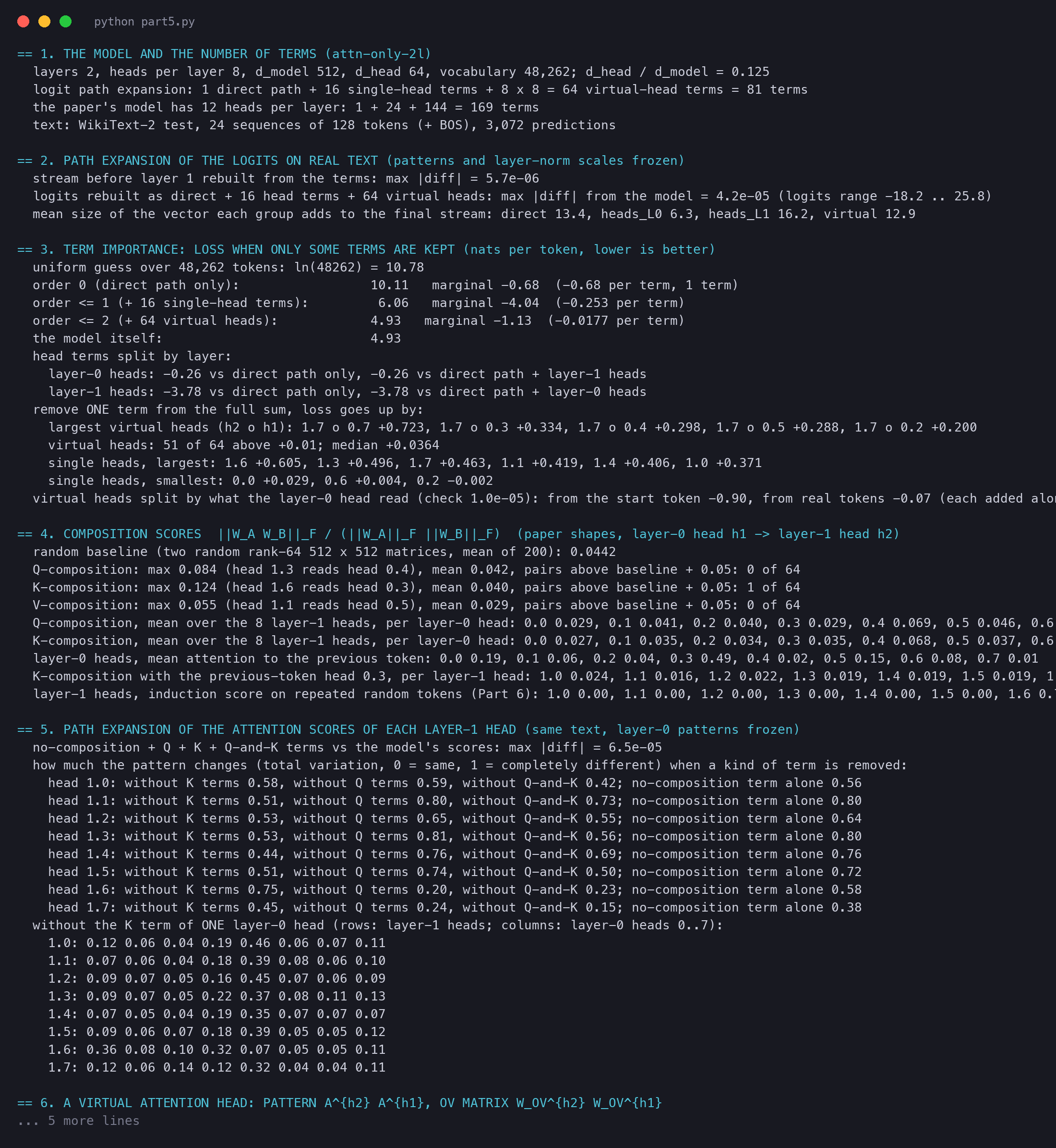
On the real model. Our script does the same on attn-only-2l, with 3,072 tokens. It keeps the attention patterns and the layer-norm scales from a normal run, and holds them fixed. Then every step is a matrix product, so the expansion is exact. It builds the direct path, the 16 single-head terms and the 64 virtual-head terms, adds them, and compares with the model:

python

o0 = [A0[:, h] @ (x0n @ W_V[0, h]) @ W_O[0, h] for h in range(8)]       # what each layer-0 head writes
virt[h2][h1] = A1[:, h2] @ (cen(o0[h1]) / s1 @ W_V[1, h2]) @ W_O[1, h2]  # layer-1 head h2 moving what h1 wrote
full = direct + sum(o0) + sum(o1_single) + sum(all virt)                # then centre, scale and unembed

plain text

== 2. PATH EXPANSION OF THE LOGITS ON REAL TEXT (patterns and layer-norm scales frozen)
  stream before layer 1 rebuilt from the terms: max |diff| = 5.7e-06
  logits rebuilt as direct + 16 head terms + 64 virtual heads: max |diff| from the model = 4.2e-05 (logits range -18.2 .. 25.8)

The 81 terms rebuild every logit to within 0.00005, on logits that run from -18.2 to 25.8. So the expansion is not an approximation. It is the model, written another way.

From the paperPath Expansion of Logits

What it says

The direct path term and the individual head terms are "identical to the one-layer model". The "virtual attention head" term corresponds to V-composition. In practice, virtual heads "tend to not play a significant role in small two-layer models".

What it means

This is a strong and useful claim. If it holds, the logits of a two-layer model look almost like those of a one-layer model. They are a bigram table plus a list of skip-trigram heads. Everything that Part 4 learned to read would still apply.

But notice what the logit equation hides. Each $A^h$ of a layer-2 head is treated as given. Where does that pattern come from? It comes from the second layer's QK circuit, and that is where Q- and K-composition live. The next section opens it.

We test the claim about virtual heads later, in the term importance section. Our model gives a more mixed answer than the paper's.

The attention scores as a sum of paths

From the paperPath Expansion of Attention Scores QK Circuit

What it says

The logit expansion "misses what is probably the most radically different property" of a two-layer model. Q- and K-composition give "much more expressive second layer attention patterns". For a first-layer head, the QK circuit is "the same matrix we saw in the one-layer model": $C_{QK}^{h\in H_1}={W_{\mathrm{E}}}^{\top}W_{\mathrm{QK}}^hW_{\mathrm{E}}$ .

What it means

A first-layer head scores pairs of plain tokens. Its question is fixed: "standing on token B, how much do I like token A?" That is the table of Part 2.

A second-layer head scores pairs of streams that layer 1 has already changed. So its question can be about more than the token itself. For example, it can look for an earlier position whose stream says "the token before me was B". That is a kind of question no one-layer head can ask. Part 6 shows that this is exactly how induction heads work.

From the paperPath Expansion of Attention Scores QK Circuit

What it says

In the first layer, $W_{\mathrm{QK}}$ acts on the token embeddings. "But by the second layer", it acts on $x_1$ , "the residual stream after first layer attention heads". The first layer sits on both the "key side" and the "query side". "Then we apply our path expansion trick to the product."

What it means

A score is a meeting of two vectors: the destination's stream (through the query) and the source's stream (through the key). In layer 2, each of those two streams is itself a sum: the embedding plus what every layer-1 head wrote.

So the score is a product of two sums. Multiply it out, and each term pairs one route on the query side with one route on the key side. That is the same trick as for the logits, applied twice.

The derivation

Write the stream at position $i$ before layer 2 as a sum of paths. It is the embedding, plus what each layer-1 head $h$ moved into position $i$ :

x_{1,i}=W_{\mathrm{E}}t_i+\sum_{h\in H_1}\sum_{i'}A^h_{ii'}\,W_{\mathrm{OV}}^hW_{\mathrm{E}}t_{i'}

Here $t_i$ is the one-hot vector of token $i$ , as in Part 2. The score of a layer-2 head $h$ for destination $i$ and source $j$ is $s_{ij}=x_{1,i}^{\top}W_{\mathrm{QK}}^hx_{1,j}$ . Put the sum in on both sides. Each side has a "direct" part and a "moved by a head" part, so the product has four groups. Write $d_i=W_{\mathrm{E}}t_i$ for the direct part and $m_i$ for the part that layer-1 heads moved in:

\begin{aligned} s_{ij}={}&d_i^{\top}W_{\mathrm{QK}}^h\,d_j+m_i^{\top}W_{\mathrm{QK}}^h\,d_j\\ &+d_i^{\top}W_{\mathrm{QK}}^h\,m_j+m_i^{\top}W_{\mathrm{QK}}^h\,m_j \end{aligned}

The first term is the no composition group: both sides are plain embeddings, as in a one-layer model. The second is the Q-composition group: a layer-1 head prepared the query: it changes what the destination is looking for. The third is the K-composition group: a layer-1 head prepared the key, which changes what each source offers. In the last group, layer 1 prepared both.

A toy example. Let the query be $q=q_d+q_h$ with a direct part $q_d=(1,0)$ and a moved part $q_h=(0,1)$ . Let the key be $k=k_d+k_h$ with $k_d=(2,1)$ and $k_h=(1,3)$ . The four terms are $q_d\cdot k_d=2$ , $q_h\cdot k_d=1$ , $q_d\cdot k_h=1$ and $q_h\cdot k_h=3$ . They add up to 7, and indeed $(1,1)\cdot(3,4)=7$ .

From the paperPath Expansion of Attention Scores QK Circuit

What it says

The expansion has to be written as a "6-dimensional tensor", because the score is a function of two streams. Each term has the form $A_q\otimes A_k\otimes W$ . Here $A_q$ "describes the movement of query-side information between tokens". $A_k$ does the same for the key side, and $W$ combines them into a score.

What it means

The notation looks heavy, but the idea is the one in our toy. Each term needs two attention patterns, not one. One says how layer 1 moved information into the destination (the query side). The other says how layer 1 moved information into the source (the key side).

In the logits, one pattern was enough, because a logit has only one position. A score has two positions, a destination and a source, so it needs one mixing matrix for each. That is why the tensor grows from two factors to three. When a side has no head on it, its factor is just $\text{Id}$ .

On the real model. Our script splits the scores of all eight layer-1 heads into these four groups, with the layer-0 patterns frozen. The groups add up to the model's scores to within 0.00007. Then it asks a functional question. If we delete one group, how much does the attention pattern change? We measure the change with the total variation distance.

plain text

  no-composition + Q + K + Q-and-K terms vs the model's scores: max |diff| = 6.5e-05
    head 1.6: without K terms 0.75, without Q terms 0.20, without Q-and-K 0.23; no-composition term alone 0.58
    head 1.7: without K terms 0.45, without Q terms 0.24, without Q-and-K 0.15; no-composition term alone 0.38

For each layer-1 head, how much its attention pattern changes when the K-composition terms are removed (orange) and when the Q-composition terms are removed (blue), on 3,072 tokens of WikiText. Head 1.6 changes by 0.75 without its K terms and only 0.20 without its Q terms.

Head 1.6 stands out. Remove its K-composition terms, and its pattern changes by 0.75, which means it now looks almost somewhere else. Remove its Q-composition terms, and it changes by only 0.20. So this head mostly relies on keys that layer 1 prepared. Part 6 shows that head 1.6 is an induction head. On repeated random tokens its induction score is 0.71, and no other head is above 0.04.

Heads 1.0 to 1.5 change a lot without either kind of term, between 0.44 and 0.81. So almost every layer-1 head uses Q- or K-composition in some way. This measure cannot say whether that use is useful for the predictions, only that the pattern depends on it.

Measuring composition from the weights

The paper then reverse-engineers one two-layer model. It starts with a map of which heads compose.

From the paperAnalyzing a Two-Layer Model

What it says

Small two-layer models often have "a very simple structure of composition". There, "the only type of composition is K-composition between a single first layer head and some of the second layer heads". That first-layer head "primarily attends to the previous token". The second-layer heads are "induction heads".

What it means

Of all the routes the expansions allow, the paper finds that its model uses very few. One first-layer head does a simple job: at each position, it copies in information about the token just before. Some second-layer heads then use that copied information in their keys.

Why would a key want to know the previous token? Because then a source position can advertise "the token before me was B". A destination standing on B can find it. Part 6 builds the full mechanism; here we only need the fact that the composition is K-composition, with one head.

From the paperAnalyzing a Two-Layer Model

What it says

Composition is measured by "the Frobenius norm of the product of the relevant matrices, divided by the norms of the individual matrices". For K-composition, the score is $\|W_{\mathrm{QK}}^{h_2}W_{\mathrm{OV}}^{h_1}\|_F/(\|W_{\mathrm{QK}}^{h_2}\|_F\|W_{\mathrm{OV}}^{h_1}\|_F)$ . Q-composition uses ${W_{\mathrm{QK}}^{h_2}}^{\top}$ , and V-composition uses $W_{\mathrm{OV}}^{h_2}$ . The paper subtracts "the empirical expected amount for random matrices of the same shapes".

What it means

The question is: how much of what head $h_1$ writes can head $h_2$ read? The product $W_{\mathrm{QK}}^{h_2}W_{\mathrm{OV}}^{h_1}$ is "first $h_1$ writes, then $h_2$ 's key reads". If $h_2$ 's key reads exactly the strip that $h_1$ writes, the product is big. If the strips are at right angles, the product is zero.

Dividing by the two norms removes plain size. A head with large weights should not look more connected only because its numbers are large. The result is a score between 0 and 1 that measures alignment, not volume.

The measure, step by step

The score for K-composition is:

\text{K-comp}(h_1,h_2)=\frac{\|W_{\mathrm{QK}}^{h_2}W_{\mathrm{OV}}^{h_1}\|_F}{\|W_{\mathrm{QK}}^{h_2}\|_F\;\|W_{\mathrm{OV}}^{h_1}\|_F}

Read it left to right. On top is the size of the combined map "head $h_1$ writes, then head $h_2$ reads the result as a key". Below are the sizes of the two maps on their own. The ratio can never be more than 1, because the norm of a product is at most the product of the norms.

A toy example. First the norm. For the matrix $\begin{bmatrix}1&2\\2&0\end{bmatrix}$ , the norm is $\sqrt{1+4+4+0}=3$ . Now take a stream of three numbers. Head 1 reads dimension 1 and writes it, doubled, into dimension 3. So its $W_{\mathrm{OV}}$ has a single entry 2, in row 3 and column 1. Head 2's query reads dimension 1 and its key reads dimension 3: $W_{\mathrm{QK}}$ has a single 1, in row 1 and column 3.

The product $W_{\mathrm{QK}}W_{\mathrm{OV}}$ has a single entry 2, so its norm is 2. The norms of the two factors are 1 and 2. The K-composition score is $2/(1\cdot2)=1$ : perfect alignment. The Q-composition score uses $W_{\mathrm{QK}}^{\top}$ , whose query side reads dimension 3. The product is zero, so the score is 0. A third head whose key reads dimension 2 also scores 0, because head 1 never writes there.

On the real model. Our script computes all three scores for all 64 pairs of heads. For the random baseline, it averages the score of 200 pairs of random 512 × 512 matrices of rank 64:

plain text

== 4. COMPOSITION SCORES  ||W_A W_B||_F / (||W_A||_F ||W_B||_F)  (paper shapes, layer-0 head h1 -> layer-1 head h2)
  random baseline (two random rank-64 512 x 512 matrices, mean of 200): 0.0442
  Q-composition: max 0.084 (head 1.3 reads head 0.4), mean 0.042, pairs above baseline + 0.05: 0 of 64
  K-composition: max 0.124 (head 1.6 reads head 0.3), mean 0.040, pairs above baseline + 0.05: 1 of 64
  V-composition: max 0.055 (head 1.1 reads head 0.5), mean 0.029, pairs above baseline + 0.05: 0 of 64
  layer-0 heads, mean attention to the previous token: 0.0 0.19, 0.1 0.06, 0.2 0.04, 0.3 0.49, 0.4 0.02, 0.5 0.15, 0.6 0.08, 0.7 0.01

Q-, K- and V-composition scores between every layer-0 head (columns) and every layer-1 head (rows) of attn-only-2l, minus the random baseline of 0.044. The brightest cell is in the K-composition map: head 1.6 reading head 0.3, with a score of 0.124. The column of head 0.4 is a little above the baseline in the Q and K maps.

The picture repeats the paper's story on a different model. Most scores sit near the random baseline of 0.044. Only one pair stands clearly above it: head 1.6 reading head 0.3, with K-composition 0.124. Head 0.3 is the head that attends most to the previous token, with a mean weight of 0.49. Head 1.6 is the induction head we met above. So the weights alone point to a previous-token head feeding the keys of an induction head.

There is a second, weaker signal in the maps: the column of head 0.4. Averaged over the eight layer-1 heads, its Q-composition is 0.069 and its K-composition 0.068. Every other layer-0 head stays at or below 0.046. No single cell of that column passes our threshold, but the whole column sits above the baseline.

The functional test of the previous section agrees. Remove the K term of head 0.4 alone, and the patterns of six layer-1 heads change by 0.35 to 0.46. Head 0.4 puts 65% of its weight on the start token, so much of what it writes is the same at every position. Many layer-1 heads seem to use that vector to tune their scores. Our tests show that they depend on it, not what they use it for.

plain text

  Q-composition, mean over the 8 layer-1 heads, per layer-0 head: 0.0 0.029, 0.1 0.041, 0.2 0.040, 0.3 0.029, 0.4 0.069, 0.5 0.046, 0.6 0.040, 0.7 0.044
  K-composition, mean over the 8 layer-1 heads, per layer-0 head: 0.0 0.027, 0.1 0.035, 0.2 0.034, 0.3 0.035, 0.4 0.068, 0.5 0.037, 0.6 0.038, 0.7 0.041

The correction

After publication, the authors found a bug that affected the composition diagram.

From the paperCorrection: Attention Head Composition Diagram

What it says

A bug in a library for low-rank matrices "only affected one diagram", but it changes the reading of the two-layer section. "In particular, there is more attention head composition going on in that model than it seemed."

What it means

The paper explains the bug in its correction notes. To save time, the library used a shortcut that is valid for traces and eigenvalues. It applied a similar shortcut to the Frobenius norm, where it is not valid. So the diagram did not measure the composition score as defined. It measured something narrower, which happens to respond very strongly to induction-head composition.

That is why the original diagram looked so clean. It filtered out most other kinds of composition. Our scores above use the correct formula: we multiply the full matrices and take the norm of the product.

Which terms matter

The paper chose to ignore the virtual heads because it saw no V-composition. It then checks that choice with an experiment.

From the paperTerm Importance Analysis

What it says

The trick is to run the model several times, "replacing the present activations with activations from previous times you ran the model". Step 1 saves all attention patterns. Step 2 freezes them and replaces every head output "with a zero tensor of the same shape". Each later step uses the outputs saved in the step before. "Freezing the attention patterns to ground truth" makes the ablation target only V-composition.

What it means

Watch what each run lets through. In step 2, every head output is zero, so only the direct path reaches the logits. That is the order-0 model. In step 3, each head gets the output it produced in step 2, which was computed from the direct path only. So paths through one head get through, and paths through two heads do not. Each new run allows one more head along a path.

The difference between the losses of two runs is the marginal effect of one order. Frozen patterns keep Q- and K-composition untouched, because the patterns already contain them.

Our script does the same thing in a different way. It already has every term from the path expansion, so it just adds up the orders it wants, and unembeds the sum. With frozen patterns and frozen layer-norm scales, this gives the same partial models.

The marginal effect of order $n$ is a simple difference:

\Delta_n=\mathcal{L}_{\le n}-\mathcal{L}_{\le n-1}

Here $\mathcal{L}_{\le n}$ is the loss when all terms up to order $n$ are kept. For order 0, the paper compares with the uniform guess. A negative $\Delta_n$ means order $n$ helps. The paper also divides by the number of terms, to get the help per term.

On the real model. Here is the same table for attn-only-2l on our 3,072 tokens:

plain text

== 3. TERM IMPORTANCE: LOSS WHEN ONLY SOME TERMS ARE KEPT (nats per token, lower is better)
  uniform guess over 48,262 tokens: ln(48262) = 10.78
  order 0 (direct path only):                 10.11   marginal -0.68  (-0.68 per term, 1 term)
  order <= 1 (+ 16 single-head terms):         6.06   marginal -4.04  (-0.253 per term)
  order <= 2 (+ 64 virtual heads):            4.93   marginal -1.13  (-0.0177 per term)
  the model itself:                           4.93

The loss drop from each order of terms. Top, the paper's model: direct path 1.8 nats, single heads 5.2, virtual heads 0.3. Bottom, our run of attn-only-2l on 3,072 WikiText tokens: direct path 0.68, single heads 4.04, virtual heads 1.13.

The broad shape is the same: the single-head terms do most of the work, with 4.04 of the 5.85 nats. The full sum gives 4.93 nats, exactly the model's own loss, which is one more check on the expansion.

Two numbers differ from the paper. The direct path helps less, only 0.68 nats. One reason is our method: the final layer-norm scale is frozen at the full model's value. A partial sum is smaller than the full stream, so its logits come out flatter. The paper does not say how it handled layer norm here.

The second difference matters more. In our model the virtual heads give 1.13 nats, not 0.3. That is nearly four times the paper's number, from fewer virtual heads (64 instead of 144). So the claim "virtual heads do not matter" does not carry over to this model as it stands. The next measurements show where this comes from.

plain text

    largest virtual heads (h2 o h1): 1.7 o 0.7 +0.723, 1.7 o 0.3 +0.334, 1.7 o 0.4 +0.298, 1.7 o 0.5 +0.288, 1.7 o 0.2 +0.200
    virtual heads: 51 of 64 above +0.01; median +0.0364
  virtual heads split by what the layer-0 head read (check 1.0e-05): from the start token -0.90, from real tokens -0.07 (each added alone to order <= 1)

Removing one virtual head at a time, the largest is 1.7 ∘ 0.7: without it, the loss rises by 0.72. All five largest run through head 1.7. Now split every layer-0 head's output into two parts: what it copied from the start token, and what it copied from real tokens. The virtual heads that start from the start token give 0.90 nats. The virtual heads that start from real tokens give only 0.07.

Adding all 64 virtual heads to the direct path and single heads lowers the loss by 1.13 nats. The part that a layer-0 head copied from the start token gives 0.90 nats. The part copied from real tokens gives only 0.07 nats.

So the large number has a plain cause. Many layer-0 heads park their attention on the start token: head 0.7 puts 60% of its weight there. The start token is the same in every sequence, so such a head writes a nearly fixed vector. Head 1.7 then moves that vector again. This acts like a learned bias delivered through two heads, not like a rule about the text. Virtual heads that carry real token information give 0.07 nats, which is close to the paper's small number.

From the paperTerm Importance Analysis

What it says

For two-layer attention-only models, we "shouldn't prioritize understanding the second order" virtual heads. We should instead "focus on the direct path" and the individual head terms. "This says nothing about Q- and K-Composition", which live in the QK circuits.

What it means

The conclusion is about where to spend effort. In the paper's model, 144 virtual heads give 0.3 nats. Reading them one by one would cost a lot and explain little.

The bracket is the important part. Removing virtual heads only tests V-composition. Q- and K-composition were never tested here, because the frozen patterns kept them. So the plan is: read the logits as one-layer terms, but read the second layer's patterns with composition in mind.

On our model, the plan needs one more step. First move the start-token path into the bias, since it carries no text. Then the conclusion holds again.

From the paperTerm Importance Analysis

What it says

The paper's first-layer heads give only 0.05 nats on top of the direct path and the second layer. On top of the direct path alone, they give 1.3 nats. The second-layer heads give 4.0 nats on top of the direct path and the first layer, and 5.2 on top of the direct path alone. "We'll focus on these."

What it means

The two numbers per row answer two questions. How much does this layer add when the other layer is already there? And how much does it add on its own? For the first layer, the answers are very different: most of what it does, the second layer can also do.

The second layer adds a lot either way. Its heads are "a lot more sophisticated", because their patterns can use the first layer through Q- and K-composition. Note that this table calls the layers 1 and 2, where the composition diagram calls them 0 and 1.

Our model shows the same split:

plain text

  head terms split by layer:
    layer-0 heads: -0.26 vs direct path only, -0.26 vs direct path + layer-1 heads
    layer-1 heads: -3.78 vs direct path only, -3.78 vs direct path + layer-0 heads

The layer-1 heads give 3.78 nats and the layer-0 heads only 0.26. In our model, the two numbers of each row happen to be almost the same. In the paper's model they differ a lot for the first layer, so there the two layers overlap in what they do.

Virtual attention heads

The paper ends the section with a closer look at the term it decided to skip.

From the paperVirtual Attention Heads

$The paragraph saying that V-Composition creates terms that act as an independent unit which performs one head operation and then the other, the composition h_2 ∘ h_1, with its own attention pattern A^{h_2}A^{h_1} and its own OV matrix W_OV^{h_2} W_OV^{h_1}$

What it says

V-composition creates terms that "operate as a kind of independent unit which performs one head operation and then the other". The result $h_2\circ h_1$ has "its own attention pattern", $A^{h_2\circ h_1}=A^{h_2}A^{h_1}$ , and "its own OV matrix", $W_{\mathrm{OV}}^{h_2\circ h_1}=W_{\mathrm{OV}}^{h_2}W_{\mathrm{OV}}^{h_1}$ . Deeper models can have higher-order virtual heads such as $h_3\circ h_2\circ h_1$ .

What it means

Think of a relay race. The first runner carries the baton from position A to position B, and the second carries it from B to C. Seen from the stands, the baton simply went from A to C. A virtual head is that A-to-C trip, seen as one move.

The formula makes it exact. The two patterns multiply, so $A^{h_2}A^{h_1}$ says where the final information came from. The two OV matrices multiply too, so $W_{\mathrm{OV}}^{h_2}W_{\mathrm{OV}}^{h_1}$ says what was carried and how it was changed on the way. The pair has exactly the shape of one head, $A\otimes W_{\mathrm{OV}}$ .

Is $A^{h_2}A^{h_1}$ really an attention pattern? Each row of $A^{h_1}$ adds up to 1, and so does each row of $A^{h_2}$ . A row of the product is a weighted average of rows of $A^{h_1}$ , with weights that add up to 1. So it also adds up to 1. And if neither head looks into the future, neither does the product. On the real model, the rows of 1.7 ∘ 0.7 add up to 1 to within 0.0000005, and its future entries are 0.

Two previous-token patterns on four tokens, and their product. In each of the first two, every token reads the one before it (token 1 reads itself). In the product, token 3 reads token 1 and token 4 reads token 2: the virtual head looks two tokens back. Every row still adds up to 1.

In our model the guess is only partly true. Head 0.0 itself puts 0.23 of its weight two tokens back, so this model does have a head that looks two back. The virtual head that looks two back the most is 1.4 ∘ 0.0, with only 0.12, and removing it costs just 0.02 nats.

plain text

  most important: 1.7 o 0.7: pattern [0.76, 0.0, 0.0, 0.0]; rows add up to 1 (max |sum - 1| 4.8e-07); future entries 0; V-composition score 0.036; removing it: loss +0.723
  most two-back: 1.4 o 0.0: pattern [0.35, 0.03, 0.09, 0.12]; rows add up to 1 (max |sum - 1| 7.2e-07); future entries 0; V-composition score 0.015; removing it: loss +0.021

Each pattern list gives the mean weight on the start token, on the token itself, one back and two back. The most important virtual head, 1.7 ∘ 0.7, puts 0.76 on the start token and almost nothing anywhere else. That is the start-token path we found above, now seen as a single virtual head.

From the paperVirtual Attention Heads

What it says

"there are a lot of virtual attention heads". The number of normal heads "grows linearly in the number of layers". The number of virtual heads of two heads "grows quadratically", of three heads cubically. "Normal attention heads are, in some sense, 'large'": one pattern and $d_\text{head}$ dimensions. That is unwieldy for small tasks, such as noticing whether a text is in the past or present tense.

What it means

Count them. With 8 heads per layer and 2 layers, our model has 16 heads and $8\times8=64$ virtual heads of order 2. The paper's model has 24 heads and 144 virtual heads. A model with 12 layers of 12 heads has 144 heads. It has $66\times144=9{,}504$ virtual heads of order 2, because there are 66 pairs of layers.

A normal head is a big tool: a full attention pattern and 64 dimensions to copy. Many jobs need far less, such as carrying one bit like "past tense". A virtual head can do such a job with a small part of two existing heads. That is why the paper expects virtual heads to matter more in larger models, even though they matter little in its small one.

The paper's next section takes up the one kind of composition that really matters in its two-layer model: the K-composition behind induction heads. That is Part 6.

Key takeaways

Composition is what a second layer adds. A later head can read what an earlier head wrote. Without it, a two-layer model is just a one-layer model with more heads.
There are three kinds. Q- and K-composition change where a head looks, through its query or its key. V-composition changes what it carries, and creates virtual heads.
The logits are a sum of paths: the direct path, one term per head, and one virtual head $(A^{h_2}A^{h_1})\otimes(W_{\mathrm{U}}W_{\mathrm{OV}}^{h_2}W_{\mathrm{OV}}^{h_1}W_{\mathrm{E}})$ per pair. On attn-only-2l, the 81 terms rebuilt the logits to within 0.00005.
A second-layer score is a sum of four groups: no composition, Q-composition, K-composition and both. Removing the K terms changed the pattern of induction head 1.6 by 0.75, and removing the Q terms by only 0.20.
Composition can be scored from the weights as a ratio of Frobenius norms. In our model, one pair stands out: K-composition 0.124 from previous-token head 0.3 to head 1.6, against a random baseline of 0.044.
The paper's composition diagram had a bug. The corrected plot keeps the main K-composition but shows more composition overall.
Single heads do most of the work. The paper: direct path 1.8, single heads 5.2, virtual heads 0.3 nats. Our model: 0.68, 4.04 and 1.13 nats, with the layer-1 heads giving 3.78 of the 4.04.
Our virtual heads mostly move the start token. They give 0.90 nats through the start token and only 0.07 through real tokens. For real text, the paper's conclusion holds.
A virtual head is a real head in disguise, with pattern $A^{h_2}A^{h_1}$ and OV matrix $W_{\mathrm{OV}}^{h_2}W_{\mathrm{OV}}^{h_1}$ . Their number grows with the square of the number of layers.

Run it yourself

The two scripts behind this part are circuits_part5.py (the path expansions, term importance, composition scores and virtual heads on attn-only-2l) and circuits_part5_toy.py (the hand-sized examples). The first one uses the WikiText-2 test set from Hugging Face and runs on the CPU in a few minutes.

bash

pip install torch datasets "transformer_lens<4"
python circuits_part5.py        # writes results/part5.json and results/part5_stdout.txt
python circuits_part5_toy.py    # writes results/part5_toy.json

Terminal output of circuits_part5.py: the model and the number of terms, the logits rebuilt from 81 paths, the losses for each order of terms, the composition scores, the four groups of attention-score terms for every layer-1 head, and two virtual heads — The real output of circuits_part5.py.

Terminal output of circuits_part5_toy.py: four paths adding up to a two-layer output, two previous-token patterns multiplying into a two-back pattern, one attention score as four terms, and composition scores on a three-dimensional stream — The real output of circuits_part5_toy.py.

The paper and the code

The paper · our scripts

Two-Layer Models: How Heads Compose

Why depth matters#

Three kinds of composition#

The logits as a sum of paths#

The derivation#

The attention scores as a sum of paths#

The derivation#

Measuring composition from the weights#

The measure, step by step#

The correction#

Which terms matter#

Virtual attention heads#

The paper and the code#

Why depth matters

Three kinds of composition

The logits as a sum of paths

The derivation

The attention scores as a sum of paths

The derivation

Measuring composition from the weights

The measure, step by step

The correction

Which terms matter

Virtual attention heads

The paper and the code