Circuits, explained · Part 7 of 7 · Covers Where Does This Leave Us?, MLP Layers, Related Work, Comments & Replications, and the later papers of 2022 to 2025

What the Paper Left Out, and What Came After

The paper's own view of its limits, the MLP layers it could not read, and the later papers that grew from it. We train a tiny model that packs five features into two numbers, and read real MLP neurons.

A Mathematical Framework for Transformer Circuits. Nelson Elhage, Neel Nanda, Catherine Olsson, Tom Henighan, Nicholas Joseph, Ben Mann, Amanda Askell, Yuntao Bai, Anna Chen, Tom Conerly, Nova DasSarma, Dawn Drain, Deep Ganguli, Zac Hatfield-Dodds, Danny Hernandez, Andy Jones, Jackson Kernion, Liane Lovitt, Kamal Ndousse, Dario Amodei, Tom Brown, Jack Clark, Jared Kaplan, Sam McCandlish, Chris Olah. Transformer Circuits Thread, 2021.

Six parts read a two-layer, attention-only model down to single heads and single paths. This last part asks what that work leaves out, and how the next four years of papers tried to fill the gap.

Where does this leave us?

The paper ends with an honest question. It studied models with no MLP layers and at most two layers. Real language models have dozens of layers, and each one has an MLP. Does anything learned here carry over?

From the paperWhere Does This Leave Us?

What it says

Normal transformers contain some circuits that are "primarily attentional". Heads still read and write the same residual stream, even when MLP layers sit between them. And "large models form many induction heads", built by "K-composition with a previous token head, just as we saw here".

What it means

Think of a big factory that adds new machines to an old line. The old conveyor belt still runs through the building, and the old machines still work. Someone who understood the small workshop can still find the belt and the old machines in the big factory.

The residual stream is that belt. Parts 1 and 2 showed that every head reads the stream with a linear map and writes back by adding. MLP layers also read and write the same stream, so they do not block the heads from each other. A path from the embedding, through two heads, to the logits still exists in a big model. It is now one path among many more.

The second claim is a promise about the next paper. The induction head of Part 6 is not a toy curiosity. The authors say they find it in large models too, built the same way. We check this promise below with the 2022 paper that delivered it.

The authors are just as clear about the limit. A large part of every real model is out of reach of these methods.

From the paperWhere Does This Leave Us?

$The paragraph saying that MLP layers make up two thirds of a standard transformer's parameters, that the fraction understood without them is even smaller than one third, and that the clearest path forward needs individually interpretable neurons, which they had limited success finding$

What it says

"MLP layers make up 2/3rds of a standard transformer's parameters." Because many heads also interact with MLP layers, the part we can understand without them is "even smaller than 1/3rd". The clearest way forward needs "individually interpretable neurons, which we've had limited success finding".

What it means

Imagine you can read one third of a book, and the other two thirds are in a code you cannot break. Worse, many sentences in your third refer to pages in the coded part. So you really understand less than a third.

The fraction is easy to check by counting weights. An attention layer has four matrices of size $d_\text{model}\times d_\text{model}$ in total. An MLP layer has two matrices of size $d_\text{model}\times 4d_\text{model}$ . That is $4d^2$ against $8d^2$ , so the MLP holds two thirds. Our count on real models below gives exactly this.

The last sentence names the real problem. To read an MLP, you want each neuron to mean one thing. The paper says such neurons were rare. The rest of this part follows that one sentence through four years of work.

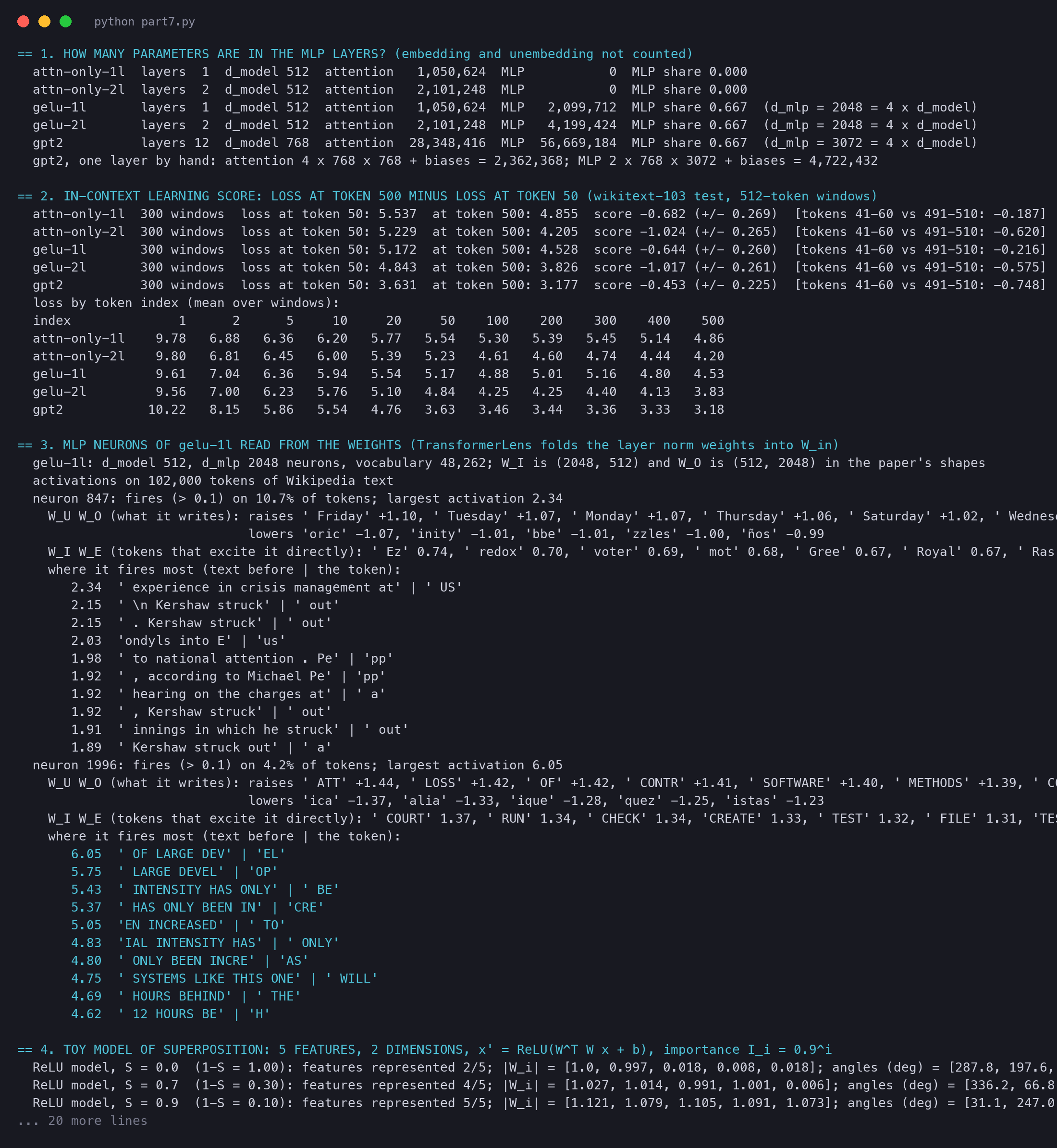
Here is the count from our script. It adds up every weight and bias inside the attention layers and inside the MLP layers, and leaves out the embedding and unembedding:

plain text

  attn-only-1l  layers  1  d_model 512  attention   1,050,624  MLP           0  MLP share 0.000
  attn-only-2l  layers  2  d_model 512  attention   2,101,248  MLP           0  MLP share 0.000
  gelu-1l       layers  1  d_model 512  attention   1,050,624  MLP   2,099,712  MLP share 0.667  (d_mlp = 2048 = 4 x d_model)
  gelu-2l       layers  2  d_model 512  attention   2,101,248  MLP   4,199,424  MLP share 0.667  (d_mlp = 2048 = 4 x d_model)
  gpt2          layers 12  d_model 768  attention  28,348,416  MLP  56,669,184  MLP share 0.667  (d_mlp = 3072 = 4 x d_model)
  gpt2, one layer by hand: attention 4 x 768 x 768 + biases = 2,362,368; MLP 2 x 768 x 3072 + biases = 4,722,432

gelu-1l and gelu-2l come from the same family as the attention-only models of this series. They add one MLP to each layer. gpt2 is the 124-million-parameter GPT-2. In all three, the MLP share is 0.667.

How the weights inside the layers split between attention and MLP. In gelu-1l, gelu-2l and gpt2 the attention layers hold one third and the MLP layers two thirds, because each MLP has four times as many neurons as the stream has dimensions.

MLP layers

The paper has a short section on MLP layers in its "Additional Intuition and Observations". It shows why the tools of Parts 3 to 6 stop working there, and which part of them still works.

From the paperMLP Layers

What it says

An MLP layer computes $a^m_\text{pre}=W_{\mathrm{I}}^m x_i$ , then $a^m=\text{GeLU}(a^m_\text{pre})$ , and adds $W_{\mathrm{O}}^m a^m$ to the stream. "The presence of the GeLU activation means we can't linearize through MLP layers as we did attention layers." Neurons were "much harder to develop hypotheses for".

What it means

Every trick of Parts 3 to 6 used one fact: once the attention pattern is fixed, a head is a product of matrices. Products of matrices can be multiplied out, and sums can be split into terms. The GeLU breaks this. It bends every number, so a sum that goes in does not come out as a sum.

The paper then gives two reasons for hope, and one for worry. Neurons have a curved function, which should push each feature onto one neuron. They are four times wider than the stream, so there is room. But in practice, most neurons did not have a clear meaning.

Here is the MLP layer as one equation, in the series notation (column vectors):

x_{i+1}=x_i+W_{\mathrm{O}}^m\,\text{GeLU}\!\left(W_{\mathrm{I}}^m\,x_i\right)

Read it from the inside out. $W_{\mathrm{I}}^m$ is the input matrix of MLP layer $m$ ; in gelu-1l it is 2,048 × 512, so it turns the 512-number stream into 2,048 pre-activations. GeLU acts on each of the 2,048 numbers alone. $W_{\mathrm{O}}^m$ is 512 × 2,048 and writes the result back. The new stream is the old stream plus that write.

Why does the bend matter so much? In Part 3 a sum of paths went into the unembedding, and each path could be studied alone. Let us try the same with the GeLU and two paths that bring $+1$ and $-1$ to one neuron. Our toy script prints:

plain text

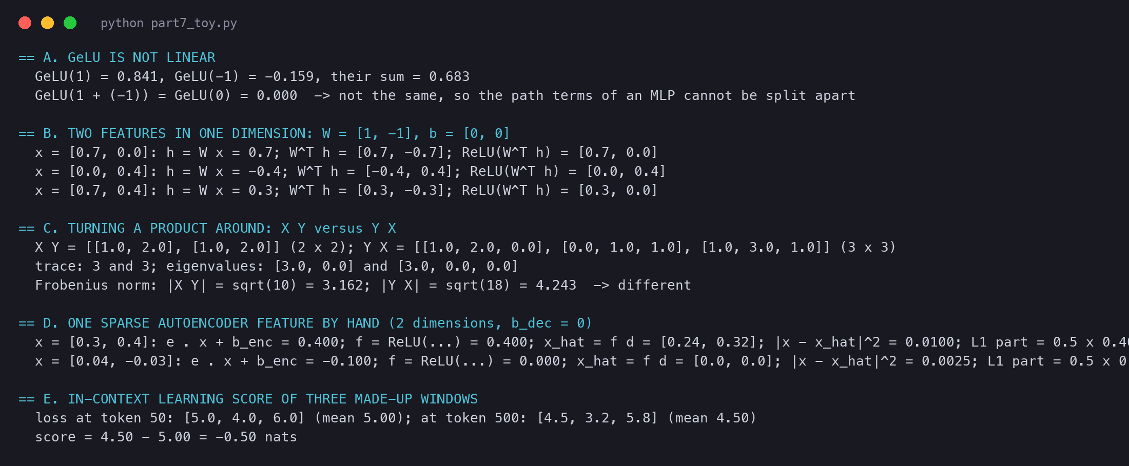
  GeLU(1) = 0.841, GeLU(-1) = -0.159, their sum = 0.683
  GeLU(1 + (-1)) = GeLU(0) = 0.000  -> not the same, so the path terms of an MLP cannot be split apart

The two paths together give 0. Taken one by one and added, they give 0.683. So the effect of one path on a neuron depends on what every other path brings. There is no clean "term" to study alone.

The part that still works: the edges of the MLP

The paper does not give up on MLP layers. It notices that the two sides of an MLP are still linear. Only the middle bends.

From the paperMLP Layers

What it says

In a one-layer model, a neuron's pre-activation gets "essentially the same equation" as the logits. It has a direct term $W_{\mathrm{I}}^m W_{\mathrm{E}}$ plus one term per head. And $W_{\mathrm{U}} W_{\mathrm{O}}^m$ "tells us how the activation of each neuron affects the logits".

What it means

Think of a neuron as a light bulb wired between two switch boards. We cannot see inside the bulb. But we can read the wires that lead into it, and the wires that lead out.

The wires in are the path expansion of Part 3, with $W_{\mathrm{I}}^m$ in place of $W_{\mathrm{U}}$ . They say which tokens, read directly or through a head, push the neuron up. The wires out are $W_{\mathrm{U}} W_{\mathrm{O}}^m$ . They say which next tokens the neuron votes for when it is on. Both can be read from the weights, with no text at all.

In symbols, with $H_1$ the heads of the only layer:

a^m_\text{pre}=W_{\mathrm{I}}^m W_{\mathrm{E}}+\sum_{h\in H_1}A^h\otimes\left(W_{\mathrm{I}}^m W_{\mathrm{OV}}^h W_{\mathrm{E}}\right)

$W_{\mathrm{I}}^m W_{\mathrm{E}}$ is a 2,048 × 48,262 table: one row per neuron, one column per token. Its entry says how much that token, at the current position, pushes that neuron through the direct path. The second term is the same with a head in between, like the OV circuit of Part 2. The direct effect of neuron $n$ on the logits is column $n$ of $W_{\mathrm{U}} W_{\mathrm{O}}^m$ , a list of 48,262 numbers, one per next token.

We read both sides for two neurons of gelu-1l. We looked at 14 neurons picked at random and chose these two because they show the two outcomes. The text comes from the test set of WikiText-103 (Wikipedia articles), 102,000 tokens in all. The library folds the layer norm weights into $W_{\mathrm{I}}$ , so the direct-path numbers are right only up to the layer norm's scale.

plain text

  neuron 847: fires (> 0.1) on 10.7% of tokens; largest activation 2.34
    W_U W_O (what it writes): raises ' Friday' +1.10, ' Tuesday' +1.07, ' Monday' +1.07, ' Thursday' +1.06, ' Saturday' +1.02, ' Wednesday' +0.99, ' September' +0.97, ' November' +0.95
    W_I W_E (tokens that excite it directly): ' Ez' 0.74, ' redox' 0.70, ' voter' 0.69, ' mot' 0.68, ' Gree' 0.67, ' Royal' 0.67, ' Ras' 0.66, ' Trading' 0.65
    where it fires most (text before | the token):
       2.34  ' experience in crisis management at' | ' US'
       2.15  ' \n Kershaw struck' | ' out'
       1.98  ' to national attention . Pe' | 'pp'
       1.92  ' hearing on the charges at' | ' a'
  neuron 1996: fires (> 0.1) on 4.2% of tokens; largest activation 6.05
    W_U W_O (what it writes): raises ' ATT' +1.44, ' LOSS' +1.42, ' OF' +1.42, ' CONTR' +1.41, ' SOFTWARE' +1.40, ' METHODS' +1.39, ' COMP' +1.39, ' GOODS' +1.38
    W_I W_E (tokens that excite it directly): ' COURT' 1.37, ' RUN' 1.34, ' CHECK' 1.34, 'CREATE' 1.33, ' TEST' 1.32, ' FILE' 1.31, 'TEST' 1.30, 'SHORT' 1.29
    where it fires most (text before | the token):
       6.05  ' OF LARGE DEV' | 'EL'
       5.75  ' LARGE DEVEL' | 'OP'

What two neurons of gelu-1l write, read from W_U W_O alone. Neuron 847 raises days of the week, Friday by 1.10 and Monday by 1.07. Neuron 1996 raises words in capital letters, ATT by 1.44 and LOSS by 1.42.

Neuron 1996 is the easy case. It fires on text in capital letters, its direct inputs are words in capitals, and it raises words in capitals. One meaning on both sides. The paper calls such a unit monosemantic.

Neuron 847 is the hard case. Its output side is clean: it votes for days of the week and months.

But its input side is a mix. It fires on " out" after "Kershaw struck", on " US" after "at", and in the middle of a name, "Pe|pp". Its direct inputs (" Ez", " redox", " voter") share nothing we can see. This is a polysemantic neuron, and it is the common case. Our sample is small, so it cannot tell how common. The later papers measure that.

What the paper says about itself

Before the later papers, two passages of the paper itself are worth reading again. They look back at the whole series.

From the paperRelated Work

What it says

"Induction heads offer an object lesson in how naive interpretation of attention patterns can both be very informative and also misleading." They are "totally reliant on a previous token head in the prior layer, through K-composition". Without that, one would "totally misunderstand the role of the previous token head".

What it means

Many earlier papers drew attention patterns and read them as explanations: "the model looked at this word". This passage says that picture is half right. The induction head's pattern does point at the token the model will copy, so it is informative.

But the pattern hides why. The head finds that token only because the head before it wrote "the previous token was A" into the stream, as Part 6 showed. Looking at the previous-token head's pattern alone, you would think it does something dull. Its real job only shows up in the K-composition term of Part 5.

So a pattern tells you where a head reads. It does not tell you how the head decided, or what other heads made that decision possible. Keep this in mind for the 2025 paper at the end of this part.

The second passage is a note the authors added more than a year later.

The same comments section has a correction that touches Part 5.

From the paperComments & Replications

What it says

A bug in their library "only affected one diagram". Still, "there is more attention head composition going on in that model than it seemed". They had "accidentally applied an analogous identity to accelerate computing the Frobenius norm".

What it means

Some quantities do not change when you turn a product of matrices around: $\text{Tr}(XY)=\text{Tr}(YX)$ , and $XY$ and $YX$ have the same nonzero eigenvalues. The size of a matrix, its Frobenius norm, is not one of them. The library treated it as if it were.

The composition scores of Part 5 are ratios of Frobenius norms. So the old diagram measured a slightly different thing. The note says the K-composition with the previous-token head is still the main effect. The correction adds that two induction heads also lean on a head that looks at the last several tokens.

A tiny example shows the trap. Take a 2 × 3 matrix $X$ and a 3 × 2 matrix $Y$ :

X=\begin{bmatrix}1&2&0\\0&1&1\end{bmatrix},\qquad Y=\begin{bmatrix}1&0\\0&1\\1&1\end{bmatrix}

The Frobenius norm is the square root of the sum of all squared entries, $\lVert M\rVert_F=\sqrt{\sum_{ij}M_{ij}^2}$ . Our toy script computes both orders:

plain text

  X Y = [[1.0, 2.0], [1.0, 2.0]] (2 x 2); Y X = [[1.0, 2.0, 0.0], [0.0, 1.0, 1.0], [1.0, 3.0, 1.0]] (3 x 3)
  trace: 3 and 3; eigenvalues: [3.0, 0.0] and [3.0, 0.0, 0.0]
  Frobenius norm: |X Y| = sqrt(10) = 3.162; |Y X| = sqrt(18) = 4.243  -> different

The trace and the nonzero eigenvalue agree, 3 and 3. The norms do not: 3.162 against 4.243. You can check $XY$ by hand: each row is $(1, 2)$ , so the squares add up to $1+4+1+4=10$ .

The next paper: induction heads in every model (2022)

The promise of "Where does this leave us?" became In-context Learning and Induction Heads, published on 8 March 2022. It moves from two-layer toys to models of many sizes, with MLPs. First it needs a definition that works without reading weights.

From the paperIn-context Learning and Induction Heads (2022)Key Concepts

What it says

An induction head shows two properties on a repeated random sequence of tokens. Prefix matching: "The head attends back to previous tokens that were followed by the current and/or recent tokens." Copying: "The head's output increases the logit corresponding to the attended-to token."

What it means

Part 6 found induction heads by reading their QK and OV circuits. That works in a two-layer model, but it is hard in a model with 40 layers and MLPs in between. So this paper defines an induction head by what it does, not by how it is built.

The test is the one Part 6 ran: random tokens, repeated twice. On the second copy, an induction head looks at the token just after the earlier copy of the current token (prefix matching). It then raises that token's logit (copying). A head that passes both tests is an induction head, whatever its weights look like.

The paper also needs a way to measure in-context learning that does not depend on a chosen task.

From the paperIn-context Learning and Induction Heads (2022)Key Concepts

What it says

The "in-context learning score" is "the loss of the 500th token in the context minus the average loss of the 50th token". It is "averaged over dataset examples". The two indices were chosen "somewhat arbitrarily".

What it means

Think of a reader who starts a novel. On page 1 they cannot guess the next word well. By page 20 they know the names, the place and the style, so their guesses improve. The score measures how much better the guesses get between an early point and a late point of the same text.

The loss at token 50 already includes what any model knows about language. The loss at token 500 adds what it picked up from the 449 tokens in between. The difference isolates the part that comes from the context.

As an equation, with $\ell_k$ the loss (in nats) of predicting token $k$ , averaged over many texts:

\text{ICL score}=\ell_{500}-\ell_{50}

A negative score means the model is better late in the text. The more negative, the more it learns from the context. A tiny example from our toy script, with three texts:

plain text

  loss at token 50: [5.0, 4.0, 6.0] (mean 5.00); at token 500: [4.5, 3.2, 5.8] (mean 4.50)
  score = 4.50 - 5.00 = -0.50 nats

The paper's central observation is about when this score appears during training.

From the paperIn-context Learning and Induction Heads (2022)Argument 1

What it says

In-context learning "develops abruptly in a narrow window early in training (roughly 2.5 to 5 billion tokens)". Before it there is "less than 0.15 nats" of it, after it "roughly 0.4 nats". This holds across model sizes, "except for the one layer model where not much in-context learning ever forms".

What it means

You might expect a skill to grow slowly as a model trains. This one does not. It switches on in a short window, and the paper calls this a "phase change". In the same window, induction heads appear and the training loss shows a small bump.

The exception is the key fact for this series. One-layer models never get the jump. Part 6 explained why: an induction head needs a previous-token head in an earlier layer, and a one-layer model has no earlier layer. The 2021 theory predicts exactly which models can make the jump.

We can measure the score on the open models of this series. We cut 300 windows of 512 tokens from the WikiText-103 test articles. Single tokens are noisy, so we also average the loss over tokens 41 to 60 and over tokens 491 to 510:

plain text

  attn-only-1l  300 windows  loss at token 50: 5.537  at token 500: 4.855  score -0.682 (+/- 0.269)  [tokens 41-60 vs 491-510: -0.187]
  attn-only-2l  300 windows  loss at token 50: 5.229  at token 500: 4.205  score -1.024 (+/- 0.265)  [tokens 41-60 vs 491-510: -0.620]
  gelu-1l       300 windows  loss at token 50: 5.172  at token 500: 4.528  score -0.644 (+/- 0.260)  [tokens 41-60 vs 491-510: -0.216]
  gelu-2l       300 windows  loss at token 50: 4.843  at token 500: 3.826  score -1.017 (+/- 0.261)  [tokens 41-60 vs 491-510: -0.575]
  gpt2          300 windows  loss at token 50: 3.631  at token 500: 3.177  score -0.453 (+/- 0.225)  [tokens 41-60 vs 491-510: -0.748]

The single-token scores have an uncertainty of about 0.27 nats, as large as the effect, so we read the averaged ones. With them the pattern is clear. Both one-layer models gain about 0.2 nats from the context (−0.187 and −0.216). Both two-layer models gain about 0.6 nats (−0.620 and −0.575), three times as much. The MLP makes almost no difference. The number of layers does.

Mean loss at each token index of 300 Wikipedia windows of 512 tokens. All four models start near 9.6 to 9.8 nats at the first token. From about token 50 on, the two-layer models (attn-only-2l and gelu-2l) keep improving more than the one-layer models. At token 500 they are at 4.20 and 3.83 nats, against 4.86 and 4.53.

Our run cannot show the phase change itself. We have only the final weights, not snapshots from training. Our numbers are also not the paper's: the text, the tokenizer and the window starts differ. The one-layer models still gain a little, which fits Part 4: their copying skip-trigrams already use the context in a simple way. The gpt2 loss uses a different tokenizer, so only its score, not its loss, compares with the others.

From the paperIn-context Learning and Induction Heads (2022)Introduction

What it says

Six lines of evidence "establish a circumstantial case that induction heads might be responsible for the majority of in-context learning". The results "are only the beginnings of evidence for such a case".

What it means

A circumstantial case is a case without a confession. The suspect was there at the right time, had the means, and nothing else fits as well. For small attention-only models the paper has more than that: knocking out the induction heads "greatly decreases" in-context learning.

For large models with MLPs, the evidence is mostly timing and correlation. The paper says so plainly, and lists other explanations it could not rule out. This honesty is a habit of the whole line of work. It is a good model for reading any claim in this field.

Toy Models of Superposition (2022)

The weakness the authors named, MLP neurons, got its own paper on 14 September 2022. It does not study a language model at all. It builds the smallest model that can show why neurons become polysemantic.

From the paperToy Models of Superposition (2022)Introduction

What it says

Train a model to store "five features of varying importance" "in two dimensions". "With dense features", it keeps an "orthogonal basis of the most important two features". But "if we make the features sparse", it stores four, then all five, at the cost of some "interference".

What it means

Picture a cupboard with only two shelves and five kinds of things to store. If you use all five every day, you keep the two most useful ones and throw the rest away. If you use each one only once a month, you can share the shelves. The chance that two things are needed on the same day is small.

That is the whole idea. A feature here is a property of the input, like "this text is French". Most features are off most of the time: they are sparse. Sparse features rarely collide, so a model can store more of them than it has dimensions. The price is a little noise when two of them happen to be on at once.

From the paperToy Models of Superposition (2022)The Superposition Hypothesis

What it says

Networks "want to represent more features than they have neurons". In $n$ dimensions there are only $n$ orthogonal directions, but about $\exp(n)$ "almost orthogonal" ones. If the original vector is sparse, it is often "possible to recover the original vector" from a smaller one.

What it means

In two dimensions you can only draw two arrows at right angles. In 1,000 dimensions you can draw a huge number of arrows that are all almost at right angles to each other. Each pair overlaps a little, but only a little.

So a model can give every feature its own direction, even with far more features than dimensions. When one feature is on, the others see a small echo of it. If few features are on at once, the echoes stay small, and a curved function can cut them off. The figure in the box shows the result: no single neuron lines up with a single feature. That is polysemanticity.

The toy model

From the paperToy Models of Superposition (2022)The Model

What it says

The model squeezes $x$ into $h=Wx$ , where "each column" $W_i$ is the direction of feature $x_i$ . It reads back with "the transpose of the same matrix" $W^T$ and adds a bias. Whether to add an activation function at the end is "critical to whether superposition occurs".

What it means

The model is a tiny compressor. It packs $n$ numbers into $m$ numbers, then tries to unpack them. It unpacks with the same matrix it packed with. So the direction of each feature is easy to read: it is column $i$ of $W$ .

The bias does two jobs. A feature the model cannot store gets its average value, which beats a guess of zero. And a negative bias can cut off the small echoes of other features. Without a final ReLU, the model is linear, and a linear model cannot cut anything off.

Here is the model as one equation, with the loss it is trained on:

x'=\text{ReLU}\!\left(W^{\top}W\,x+b\right),\qquad \mathcal{L}=\sum_{x}\sum_{i} I_i\,(x_i-x'_i)^2

Read it left to right. $x$ has $n$ features, $W$ is $m\times n$ , so $Wx$ is the small $m$ -number hidden vector $h$ . $W^{\top}h$ unpacks it back to $n$ numbers, $b$ is a bias per feature, and ReLU sets negative values to zero. The loss compares the output $x'$ with the input $x$ . Each error is weighted by the feature's importance $I_i$ .

The smallest case shows why the ReLU matters. Put two features into one dimension, pointing in opposite directions: $W=[1,\;-1]$ and $b=0$ . Our toy script feeds three inputs:

plain text

  x = [0.7, 0.0]: h = W x = 0.7; W^T h = [0.7, -0.7]; ReLU(W^T h) = [0.7, 0.0]
  x = [0.0, 0.4]: h = W x = -0.4; W^T h = [-0.4, 0.4]; ReLU(W^T h) = [0.0, 0.4]
  x = [0.7, 0.4]: h = W x = 0.3; W^T h = [0.3, -0.3]; ReLU(W^T h) = [0.3, 0.0]

When one feature is on, the ReLU output is perfect: two features from one number. Without the ReLU, the first input would come back as $(0.7, -0.7)$ , with a wrong −0.7. The third line is the price. When both are on, they cancel inside $h$ , and the output is wrong. If both are rarely on together, the price is rarely paid.

Now the real experiment. We trained the model with $n=5$ features, $m=2$ dimensions and importances $I_i=0.9^i$ , at four sparsities. Each run is the best of three random starts:

plain text

  ReLU model, S = 0.0  (1-S = 1.00): features represented 2/5; |W_i| = [1.0, 0.997, 0.018, 0.008, 0.018]; angles (deg) = [287.8, 197.6, 174.7, 63.4, 273.5]; b = [-0.004, -0.007, 0.496, 0.502, 0.505]; loss 0.1830
  ReLU model, S = 0.7  (1-S = 0.30): features represented 4/5; |W_i| = [1.027, 1.014, 0.991, 1.001, 0.006]; angles (deg) = [336.2, 66.8, 156.7, 246.4, 336.2]; b = [0.012, 0.013, 0.021, 0.02, 0.151]; loss 0.1019
  ReLU model, S = 0.9  (1-S = 0.10): features represented 5/5; |W_i| = [1.121, 1.079, 1.105, 1.091, 1.073]; angles (deg) = [31.1, 247.0, 104.5, 319.1, 175.8]; b = [-0.207, -0.212, -0.207, -0.205, -0.211]; loss 0.0217
  linear model, S = 0.9: features represented 2/5; |W_i| = [1.0, 1.0, 0.037, 0.02, 0.015]; angles = [357.9, 267.9, 220.7, 92.8, 220.5]; loss 0.0676

The columns W_i of our trained toy models, drawn in their two dimensions. Dense, with a ReLU: features 1 and 2 at right angles, the rest near zero. S = 0.7: four features in two opposite pairs. S = 0.9: all five as a pentagon, about 72 degrees apart. The linear model at S = 0.9 keeps only two.

Our run reproduces the paper's figure. With dense features, only features 1 and 2 have length near 1, and they sit 90.2° apart. The three others get a bias of about 0.5, which is the average of a number drawn evenly from 0 to 1. This is the "expected value" job of the bias. At $S=0.7$ , four features are stored as two opposite pairs: 336.2° and 156.7°, then 66.8° and 246.4°.

At $S=0.9$ , all five are stored. Sorted by angle they sit at 31.1°, 104.5°, 175.8°, 247.0° and 319.1°, gaps of 71° to 73°: a pentagon. Every bias is now about −0.21, the noise filter. Feature 1's neighbours echo it with 0.35 and 0.38 in $W^{\top}W$ , so after the bias of about −0.21 only 0.14 to 0.18 leaks through. The linear model at the same sparsity keeps only two features, and its loss is three times higher (0.0676 against 0.0217).

Towards Monosemanticity (2023)

If features hide in superposition, then neurons are the wrong units to read. The paper of 4 October 2023 tries to recover the features themselves, in a real model.

The equations are clearest in the 2024 paper, which uses the same design:

From the paperScaling Monosemanticity (2024)Sparse Autoencoders

What it says

Each feature has an activation $f_i(\mathbf{x})=\text{ReLU}(\mathbf{W}^{enc}_{i,\cdot}\cdot\mathbf{x}+b^{enc}_i)$ . The input is rebuilt as $\hat{\mathbf{x}}=\mathbf{b}^{dec}+\sum_i f_i(\mathbf{x})\,\mathbf{W}^{dec}_{\cdot,i}$ . The loss is the reconstruction error plus an "L1 penalty on feature activations".

What it means

The encoder asks, for each feature: how much does this activation point along my direction? If the answer is above a threshold, the feature turns on. The decoder rebuilds the activation as a sum of feature directions, each scaled by how much its feature is on.

The loss pulls two ways. The first part wants a perfect copy. The second part charges for every feature that is on. Together they ask: explain this activation with as few features as possible. That is exactly how superposition was built, run in reverse.

Here are the three equations in one place:

\begin{aligned} f_i(\mathbf{x})&=\text{ReLU}\!\left(\mathbf{W}^{enc}_{i,\cdot}\cdot\mathbf{x}+b^{enc}_i\right)\\ \hat{\mathbf{x}}&=\mathbf{b}^{dec}+\sum_{i=1}^{F}f_i(\mathbf{x})\,\mathbf{W}^{dec}_{\cdot,i}\\ \mathcal{L}&=\mathbb{E}_{\mathbf{x}}\Big[\lVert\mathbf{x}-\hat{\mathbf{x}}\rVert_2^2+\lambda\sum_i f_i(\mathbf{x})\,\lVert\mathbf{W}^{dec}_{\cdot,i}\rVert_2\Big] \end{aligned}

$\mathbf{x}$ is the activation vector with $D$ numbers. $\mathbf{W}^{enc}$ is $F\times D$ , one row per feature, and $\mathbf{W}^{dec}$ is $D\times F$ , one column (a direction) per feature. $F$ is much larger than $D$ . $\lambda$ sets the price of a feature being on. The factor $\lVert\mathbf{W}^{dec}_{\cdot,i}\rVert_2$ stops the network from cheating by making $f_i$ tiny and its direction huge.

A tiny example by hand, in two dimensions with one feature. Its direction is $d=(0.6, 0.8)$ , its encoder row is the same, $b^{enc}=-0.1$ , $b^{dec}=0$ and $\lambda=0.5$ :

plain text

  x = [0.3, 0.4]: e . x + b_enc = 0.400; f = ReLU(...) = 0.400; x_hat = f d = [0.24, 0.32]; |x - x_hat|^2 = 0.0100; L1 part = 0.5 x 0.400 = 0.200
  x = [0.04, -0.03]: e . x + b_enc = -0.100; f = ReLU(...) = 0.000; x_hat = f d = [0.0, 0.0]; |x - x_hat|^2 = 0.0025; L1 part = 0.5 x 0.000 = 0.000

The first input lies along $d$ : $0.6\times0.3+0.8\times0.4=0.5$ , minus 0.1 gives 0.4, so the feature turns on. The rebuilt vector is a little short, because the bias shrank it; that is the small price of the threshold. The second input points across $d$ , so the feature stays off. Its small error, 0.0025, is cheaper than turning a feature on.

Our test: can an autoencoder undo superposition?

The toy model gives us something real models never give: the true feature directions. So we can check an autoencoder against the truth. We trained a bigger toy model, 40 features in 10 dimensions, each feature off 95% of the time. Then we trained a sparse autoencoder with 40 features on its 10-number hidden vectors:

plain text

  toy model: 40 of 40 features represented (|W_i| > 0.5) in 10 dimensions; loss 0.1525
  features that move each of the 10 neurons by more than 0.3: [18, 17, 15, 18, 16, 14, 17, 21, 16, 17]
  best |cosine| between a feature direction and any single neuron: median 0.578, largest 0.927  (1 would mean "this neuron is this feature")
  sparse autoencoder: 40 features, L1 weight 0.3, 15,000 steps of 4,096 hidden vectors
  true features with a learned direction at cosine > 0.99: 32 of 40; > 0.9: 34 of 40; median best cosine 0.9982; worst 0.612
  the reconstruction keeps 82.8% of the variance of h; on average 1.99 true features are on per input, and the autoencoder turns on 2.86 of its features

The toy model stores all 40 features in 10 dimensions. Each of its 10 hidden units is moved strongly by 14 to 21 features, so every unit is polysemantic. The best match between a feature and a single unit has a median cosine of only 0.578.

The autoencoder does much better. For 32 of the 40 true features it found a direction at cosine above 0.99, with a median of 0.9982. Six features it did not find well; the worst match is 0.612. And it paid for sparsity: it keeps 82.8% of the variance, and turns on 2.86 features per input where 1.99 are really on. These are the same trade-offs the papers report at a vastly larger scale.

Scaling Monosemanticity (2024)

The 2023 paper worked on a one-layer model. The open question was whether the method scales. The paper of 21 May 2024 applied it to Anthropic's medium-sized production model of the time.

The features turned out to be strikingly specific, and they could be used to steer the model.

Circuit tracing (2025)

Features are the parts. The 2021 paper was about how parts connect: circuits. Two papers of 27 March 2025 bring the two together. Circuit Tracing gives the method, and On the Biology of a Large Language Model shows what it finds.

From the paperCircuit Tracing (2025)Introduction

What it says

"for a specific input, the direct interactions between features are linear", because "we freeze attention patterns and normalization denominators". The citation, number 18, is A Mathematical Framework for Transformer Circuits.

What it means

This is the "freezing attention patterns" trick of Part 3, four years later. Fix the patterns that one prompt produced. Then every path between two features is a product of matrices again, and the path expansion works.

The new piece replaces the MLPs. A transcoder is an autoencoder that reads the stream before an MLP and predicts the MLP's output from sparse features. Its features take the place of the neurons. Since they are trained to be sparse and readable, the bend of the GeLU no longer hides the meaning.

The companion paper uses these graphs to watch a model reason.

From the paperOn the Biology of a Large Language Model (2025)Multi-step Reasoning

What it says

For "Fact: the capital of the state containing Dallas is", the model answers "Austin". This needs two steps, "first, inferring that the state containing Dallas is Texas", then the capital of Texas. The paper finds "genuine two-step reasoning internally", next to a shortcut.

What it means

The word "Texas" never appears in the prompt or the answer. If the model uses it, it must exist only inside. The attribution graph shows "Dallas" features turning on a group of "Texas" features, which then push "Austin". When the paper turns the "Dallas" features down, the "Texas" features weaken too.

In 2021 the main mechanism read from weights was a two-head induction circuit in a toy model. Here, in a production model, a hidden middle step of a fact lookup can be seen and changed. That is how far the program came in four years.

The method also has a blind spot, and it is one this series knows well.

From the paperCircuit Tracing (2025)Example: Induction

What it says

On "a humble 2-layer attention-only model", with the prompt "I always loved visiting Aunt Sally. Whenever I was feeling sad, Aunt", the graph says only that "Sally" was predicted because "Sally" appeared earlier. "This misses the entire interesting story!" The head attends to "Sally" "because it was preceded by" "Aunt".

What it means

Freezing the attention patterns makes the math linear, but it throws away the QK circuit. The graph sees the OV side: a "Sally" was read and copied. It cannot see why the head looked at "Sally". That reason is the K-composition with a previous-token head, the heart of Part 6.

The authors call this "a kind of regression": the 2021 method explained it, and the 2025 method does not. It is the warning of the attention-patterns box above, come true. The two tools see different halves of the same circuit.

We ran this exact prompt on our two attention-only models:

plain text

  attn-only-1l: tokens 15; next-token top 5: ' Sally' 0.294, 'ie' 0.144, ' Mary' 0.028, ' Sue' 0.025, ' I' 0.012
    P(" Sally") = 0.294 (rank 1); strongest head of layer 0 on " Sally": 0.3 with weight 0.28
  attn-only-2l: tokens 15; next-token top 5: ' Sally' 0.779, 'ie' 0.015, ' Susan' 0.009, ' Sue' 0.009, ' Mary' 0.006
    P(" Sally") = 0.779 (rank 1); strongest head of layer 1 on " Sally": 1.6 with weight 0.40

Both models guess " Sally". The two-layer model is far more sure: 0.779 against 0.294. In its second layer, head 1.6 puts 0.40 of the last token's attention on " Sally". The one-layer model gets there another way. Its copying head 0.3 from Part 2 also reads " Sally" (weight 0.28), as a skip-trigram of Part 4: "Sally … Aunt → Sally".

This is the attention-pattern lesson in miniature. Both models look at " Sally", and an attribution graph would show both as "read Sally, say Sally". Only the QK circuits tell the two stories apart. Our run does not test which head of attn-only-2l is an induction head; that is the test of Part 6.

The series in one page

Seven parts, one idea: a transformer can be multiplied out into pieces, and the pieces can be read.

Part 1 showed the residual stream as a shared channel. Every layer reads with a linear map and writes by adding, so layers that never touch still talk through virtual weights. A zero-layer model is only a table of word pairs, $W_{\mathrm{U}} W_{\mathrm{E}}$ .

Part 2 opened one head. Its four matrices collapse into two: $W_{\mathrm{QK}}$ decides where to read, and $W_{\mathrm{OV}}$ decides what to move. Read through the embedding and unembedding, they become the QK and OV circuits, tables of tokens.

Part 3 froze the attention patterns and multiplied out a one-layer model. The logits became a direct path plus one term per head. Part 4 read those terms as skip-trigrams, found copying heads, and showed where the tables fail.

Part 5 added a second layer. Heads can compose through their queries, keys or values, and the path expansion grows terms for each pair. Part 6 found the circuit that matters most: a previous-token head feeding an induction head by K-composition. It lets a model repeat what it has seen.

This part followed the open end. MLP layers hold two thirds of the weights and do not multiply out. Superposition explains why their neurons are hard to read. Sparse autoencoders and transcoders recover readable features, and attribution graphs connect them with the same virtual weights and frozen patterns this paper introduced. And the 2025 method still needs the 2021 one to see why an induction head looks where it does.

Key takeaways

The paper names its own limit. MLP layers hold two thirds of a standard transformer's weights. Our count gives 0.667 for gelu-1l, gelu-2l and gpt2.
The GeLU breaks the path expansion. GeLU(1) + GeLU(−1) = 0.683, but GeLU(0) = 0, so paths into a neuron cannot be studied one by one.
The edges of an MLP are still linear. $W_{\mathrm{I}}^m W_{\mathrm{E}}$ says which tokens excite a neuron, and $W_{\mathrm{U}} W_{\mathrm{O}}^m$ what it writes. Neuron 1996 of gelu-1l is clean (capital letters); neuron 847 writes days of the week but fires on unrelated text.
Induction heads are in every model with two or more layers (2022). In-context learning appears in a short window of training, with the induction heads. On Wikipedia text, our two-layer models gain about 0.6 nats from the context, one-layer models about 0.2.
Superposition (2022): a model can store more sparse features than it has dimensions. Our toy model stores 2, 4, then 5 features in 2 dimensions as sparsity grows, ending as a pentagon 72° apart.
Sparse autoencoders (2023, 2024) undo superposition. On our 40-feature toy, an autoencoder found 32 of the 40 true directions at cosine above 0.99, while single units matched at a median of 0.578.
Circuit tracing (2025) reuses the paper's tools, frozen attention patterns and virtual weights, with transcoder features in place of neurons. It finds hidden steps such as "Texas" between "Dallas" and "Austin".
It cannot see QK circuits. On the "Aunt Sally" prompt it misses why the induction head looks at "Sally": the K-composition of Part 6.

Run it yourself

The two scripts behind this part are circuits_part7.py (the parameter count, the in-context learning score, the two MLP neurons, both toy models of superposition, the sparse autoencoder and the "Aunt Sally" prompt) and circuits_part7_toy.py (the hand-sized examples). The first one downloads gelu-1l, gelu-2l and gpt2 the first time, and reads the WikiText-103 test set (Salesforce/wikitext on Hugging Face). It runs on the CPU in about ten minutes. The screenshots of the later papers come from shots_part7_later.mjs.

bash

pip install torch pandas pyarrow "transformer_lens<4"
python circuits_part7.py        # writes results/part7.json and results/part7_stdout.txt
python circuits_part7_toy.py    # writes results/part7_toy.json

Terminal output of circuits_part7.py: the parameter counts, the in-context learning scores and the loss by token index, and the two MLP neurons of gelu-1l — The first 60 lines of the output of circuits_part7.py.

Terminal output of circuits_part7_toy.py: GeLU is not linear, two features in one dimension, the trace and Frobenius norm of X Y and Y X, one sparse autoencoder feature by hand, and the in-context learning score of three windows — The output of circuits_part7_toy.py.

The paper and the code

A Mathematical Framework for Transformer Circuits (2021) · the later papers · our scripts

What the Paper Left Out, and What Came After

Where does this leave us?#

MLP layers#

The part that still works: the edges of the MLP#

What the paper says about itself#

The next paper: induction heads in every model (2022)#

Toy Models of Superposition (2022)#

The toy model#

Towards Monosemanticity (2023)#

Our test: can an autoencoder undo superposition?#

Scaling Monosemanticity (2024)#

Circuit tracing (2025)#

The series in one page#

The paper and the code#

Where does this leave us?

MLP layers

The part that still works: the edges of the MLP

What the paper says about itself

The next paper: induction heads in every model (2022)

Toy Models of Superposition (2022)

The toy model

Towards Monosemanticity (2023)

Our test: can an autoencoder undo superposition?

Scaling Monosemanticity (2024)

Circuit tracing (2025)

The series in one page

The paper and the code