Circuits, explained · Part 4 of 7 · Covers Splitting Attention Head terms into Query-Key and Output-Value Circuits, Interpretation as Skip-Trigrams, Summarizing OV/QK Matrices, Do We Fully Understand One-Layer Models?

One-Layer Models: Skip-Trigrams, Copying and Their Bugs

What a one-layer attention-only model really learns, read from its weights: skip-trigrams, copying, heads that only look at position, the bugs of a factored form, and eigenvalues as a test for copying.

A Mathematical Framework for Transformer Circuits. Nelson Elhage, Neel Nanda, Catherine Olsson, Tom Henighan, Nicholas Joseph, Ben Mann, Amanda Askell, Yuntao Bai, Anna Chen, Tom Conerly, Nova DasSarma, Dawn Drain, Deep Ganguli, Zac Hatfield-Dodds, Danny Hernandez, Andy Jones, Jackson Kernion, Liane Lovitt, Kamal Ndousse, Dario Amodei, Tom Brown, Jack Clark, Jared Kaplan, Sam McCandlish, Chris Olah. Transformer Circuits Thread, 2021.

A one-layer attention-only model looks like a black box, but the paper shows that it is a very large table of word patterns. We read that table out of the weights of a real model, and find both what it does well and the mistakes it cannot avoid.

The two circuits of every head

Part 3 wrote the logits of a one-layer model as a sum of separate terms. One term is the direct path from Part 1: the bigram table $W_{\mathrm{U}} W_{\mathrm{E}}$ . Then there is one term for each head. Here is the term of head $h$ , in the paper's notation:

A^h\otimes\big(W_{\mathrm{U}} W_{\mathrm{OV}}^h W_{\mathrm{E}}\big),\qquad A^h=\text{softmax}^*\big(t^\top {W_{\mathrm{E}}}^{\top} W_{\mathrm{QK}}^h W_{\mathrm{E}}\,t\big)

Read it from the inside. The vector $t$ holds the tokens of the text, one one-hot vector per position. The matrix $A^h$ is the attention pattern of the head: which position reads which. The bracket on the left is what reading a token does to the logits. So the term says: "read some earlier tokens with weights $A^h$ , and let each token you read change the logits through one fixed table."

Part 2 met the two tables inside this formula. The paper now names them and makes them the main object of study.

From the paperSplitting Attention Head terms into Query-Key and Output-Value Circuits

What it says

Each head term contains "two separable operations", two matrices of size $n_\text{vocab}\times n_\text{vocab}$ . The QK circuit ${W_{\mathrm{E}}}^{\top} W_{\mathrm{QK}}^h W_{\mathrm{E}}$ scores every pair of tokens: "how much a given query token 'wants' to attend" to a key token. The OV circuit $W_{\mathrm{U}} W_{\mathrm{OV}}^h W_{\mathrm{E}}$ describes "how a given token will affect the output logits if attended to".

What it means

Think of a head as a reader with two cards. The first card lists preferences: "standing on in, I look back at place names". The second lists reactions: "reading Paris, I say Paris and France louder". The QK circuit is the first card, the OV circuit the second.

Both cards have a token on each side, one row and one column per token of the vocabulary. Our model has 48,262 tokens, so each card has 48,262 × 48,262 entries.

The important word is "separable". The two cards do not talk to each other. One decides where to look, and the other decides what to say about what was seen. The rest of this part shows that this simple fact explains both the strength and the bugs of one-layer models.

The paper then adds one sentence that is easy to read past. It is the key to the bugs later in this part.

From the paperSplitting Attention Head terms into Query-Key and Output-Value Circuits

What it says

The attention pattern depends on both the source and the destination token. But once the destination has decided how much to attend, "the effect on the output is solely a function of that source token".

What it means

Picture a radio station that plays a song when a listener calls. The listener decides whether to call and how loud to turn the volume. But the song is the same for every listener. Only the volume changes.

In a head, the destination token is the listener and the source token is the song. The destination only controls one number: the attention weight. What the source then adds to the logits is always the same column of the OV circuit, scaled by that weight. Keep this picture in mind. We come back to it when we look at bugs.

Part 3 also explains why we may study the two circuits apart: freeze the attention pattern, and the rest of the model is linear. Here we use the two circuits as tables and read them.

Skip-trigrams

Part 1 showed that a model with zero layers can only learn bigrams: "after token A, token B is likely". A one-layer model can do more. The paper gives the new pattern a name.

From the paperInterpretation as Skip-Trigrams

What it says

After the QK and OV circuits are multiplied out, the parameters are "simple linear or bilinear functions on tokens". The QK circuit decides which source token the destination attends back to. The OV circuit decides the effect on the prediction of the next token. "Together, the three tokens involved form a 'skip-trigram' of the form [source]... [destination][out]".

What it means

A head works at one position, the destination: the token we are standing on. It looks back and reads an earlier token, the source. Then it changes the guess for the next token, the out token. Three tokens, one rule.

Why "skip"? A normal trigram needs its three tokens side by side. Here the source can be 2 tokens back or 200 tokens back; attention reaches it either way. The skip is the gap between source and destination.

Here is one skip-trigram at work in our model, attn-only-1l. The prompt ends with a quote mark and the letter "R". Without a space in front, the name "Ralph" is cut into two tokens, "R" and "alph". We come back to this later in the part.

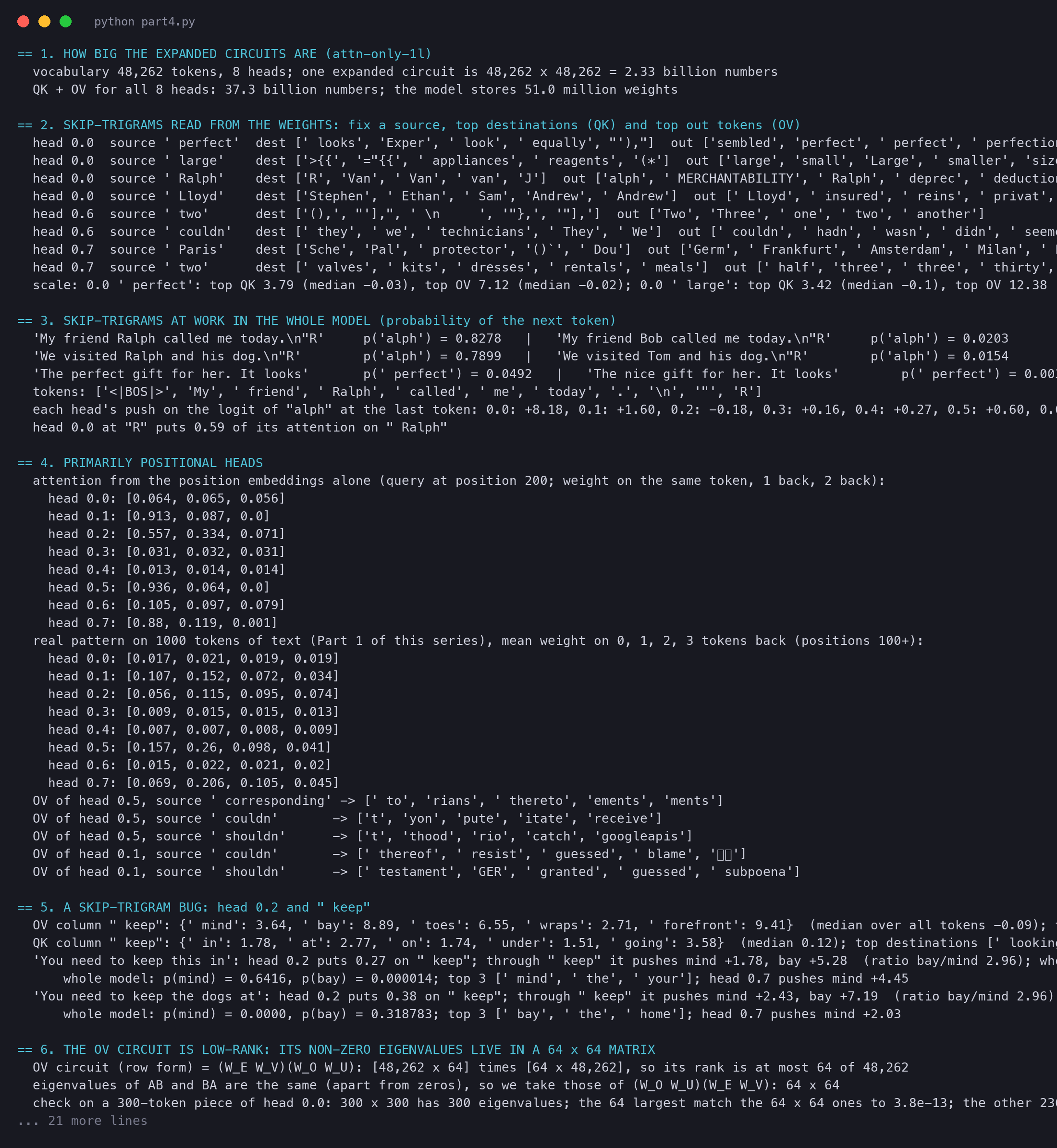
The prompt "My friend Ralph called me today", a new line, a quote mark and "R". Head 0.0 stands on the last token "R" (the destination). Its QK side reads back to " Ralph" (the source) with weight 0.59. Its OV side then raises the logit of the piece "alph" (the out token) by 8.18.

How much does a source push an out token? Use the radio picture: the volume times the song. Write $a$ for the source, $b$ for the destination and $c$ for the out token:

\Delta\,\text{logit}_c=A^h_{b\leftarrow a}\;M^h_{c,a},\qquad M^h=W_{\mathrm{U}} W_{\mathrm{OV}}^h W_{\mathrm{E}}

Read it left to right. $\Delta\,\text{logit}_c$ is how much the head raises the logit of token $c$ . $A^h_{b\leftarrow a}$ is the attention weight from the destination to the source; it comes from the QK circuit through the softmax. $M^h_{c,a}$ is one entry of the OV circuit: row $c$ , column $a$ . If a head reads several earlier tokens, their pushes add up.

A tiny example. Say the head gives weight 0.5 to the source, and the OV entry is 4. The push on the out token is $0.5\times4=2$ . If the head gives weight 0.1 to the same source, the push is $0.4$ . The volume changes, the song does not.

On the real model. On our prompt, head 0.0 at "R" gives 0.59 of its attention to " Ralph". The whole head raises the logit of "alph" by 8.18. The other seven heads add between −0.24 and +1.67. This is our script's output:

plain text

  tokens: ['<|BOS|>', 'My', ' friend', ' Ralph', ' called', ' me', ' today', '.', '\n', '"', 'R']
  each head's push on the logit of "alph" at the last token: 0.0: +8.18, 0.1: +1.60, 0.2: -0.18, 0.3: +0.16, 0.4: +0.27, 0.5: +0.60, 0.6: +1.67, 0.7: -0.24
  head 0.0 at "R" puts 0.59 of its attention on " Ralph"

A giant pile of cards

The paper then warns that "readable" does not mean "easy".

From the paperInterpretation as Skip-Trigrams

What it says

Interpretation is not trivial. A single expanded OV matrix has about 2.5 billion entries. The model is "a compressed Chinese room", and "we're left with a giant pile of cards". There is also "fungibility between variables": one head may do nothing for a token because another head already does the job. And "QK weights aren't comparable between different query vectors".

What it means

The yellow box below explains the Chinese room. The paper's point is this: we opened the room, and we found the rule cards. Each card is simple. But there are billions of them, and no one can read billions of cards.

"Fungibility" is a word from economics: one dollar note can replace another. Here it means that two heads can share a job in many ways. If head A handles a pattern, head B may show a zero for it. A zero in one table does not mean the model ignores the pattern.

The last warning matters when we rank entries. Each destination gets its own softmax, so a score of 3 may win in one row and lose in another. The top entries of a QK column are hints, not exact rankings.

How big is the pile for our model? Our script counts it:

plain text

== 1. HOW BIG THE EXPANDED CIRCUITS ARE (attn-only-1l)
  vocabulary 48,262 tokens, 8 heads; one expanded circuit is 48,262 x 48,262 = 2.33 billion numbers
  QK + OV for all 8 heads: 37.3 billion numbers; the model stores 51.0 million weights

The model stores 51.0 million numbers. Written out as cards, the same model is 37.3 billion numbers, more than 700 times as many. Nothing new was added. The cards are a different way to write the same weights, and a much longer one.

Copying

With the cards in hand, the paper looks at the largest entries. The first thing it finds is copying.

From the paperCopying / Primitive In-Context Learning

$The paragraph saying that most heads in one-layer models dedicate an enormous fraction of their capacity to copying: the OV circuit makes an attended token raise its own probability, and the QK circuit only attends back to tokens which could plausibly be next$

What it says

"most attention heads in one layer models dedicate an enormous fraction of their capacity to copying". The OV circuit makes a token, if attended to, "increase the probability of that token", and of similar tokens. The QK circuit "only attends back to tokens which could plausibly be the next token". So tokens are copied, but "only to places where bigram-ish statistics make them seem plausible".

What it means

Copying is the cheapest useful trick for a text model. Words repeat. If a story mentions "Ralph" once, "Ralph" will probably come again. A head that says "whatever I read, predict it again" wins often.

But copying blindly would be silly. After "the", a name can come, but after "Ralph" another "Ralph" rarely follows at once. So the QK circuit adds a filter: stand only on tokens after which the copied word fits. "Bigram-ish statistics" means exactly this: is "destination, then source" a pair that often appears in text?

The two cards share the work. The OV card says "repeat what you read". The QK card says "read only words that could come next here".

The paper shows examples as a table. Each row fixes one source token. It lists the destinations that attend to it most (QK) and the out tokens it raises most (OV).

From the paperCopying / Primitive In-Context Learning

What it says

For each source token, the table shows the top destination tokens and the top out tokens, and two example skip-trigrams. Examples: "perfect... are perfect", "large... contains small", "two... One two". lambda... $\\lambda seems to be the model learning LaTeX. nbsp... >&nbsp seems to be the model learning HTML escape codes.

What it means

Read one row at a time, left to right. Take the row "two". Say " two" appeared earlier, and the model now stands on " One" or " has". Then the head raises " two", " three" and " four". The out column holds the copied word and its cousins.

The LaTeX row is a nice surprise. In LaTeX, Greek letters are written with a backslash: \lambda. When the model stands on a backslash and "lambda" appeared earlier, it predicts "lambda" again. A very specific habit of a typesetting language fell out of a general copying rule.

We can make this table for our own model. For each source token, our script takes one column of each circuit of a head and lists the top entries. As in Part 2, positions and biases are left out.

plain text

== 2. SKIP-TRIGRAMS READ FROM THE WEIGHTS: fix a source, top destinations (QK) and top out tokens (OV)
  head 0.0  source ' perfect'  dest [' looks', 'Exper', ' look', ' equally', "'),"]  out ['sembled', 'perfect', ' perfect', ' perfection', 'Perfect']
  head 0.0  source ' Ralph'    dest ['R', 'Van', ' Van', ' van', 'J']  out ['alph', ' MERCHANTABILITY', ' Ralph', ' deprec', ' deduction']
  head 0.6  source ' couldn'   dest [' they', ' we', ' technicians', ' They', ' We']  out [' couldn', ' hadn', ' wasn', ' didn', ' seemed']
  head 0.7  source ' Paris'    dest ['Sche', 'Pal', ' protector', '()`', ' Dou']  out ['Germ', ' Frankfurt', ' Amsterdam', ' Milan', ' Lyon']

Our version of the paper's table, for attn-only-1l. Head 0.0 reads " perfect" and raises "perfect"; it reads " Ralph" and raises "alph". Head 0.6 reads " couldn" from " they" or " we" and raises " couldn", " hadn", " wasn". Head 0.7 reads " Paris" and raises other cities, such as Frankfurt and Amsterdam.

Several rows look like the paper's. Head 0.0 reads " perfect" from the destination " looks" and raises " perfect": "a perfect ... looks perfect". It reads " large" and raises "large" and "small", the same pair as in the paper (that row of our output is in the full log). Head 0.6 raises " couldn" and its cousins " hadn", " wasn", " didn". Head 0.7 does not copy the word itself. It reads " Paris" and raises other European cities.

The destination columns are noisier. Some make sense (" they" and " we" before " couldn"), and some are pieces of code. This is the warning of the last box: scores of different destinations are not on one scale.

Does the copying show in the predictions of the whole model? We changed one word of a prompt and measured the probability of the next token:

plain text

== 3. SKIP-TRIGRAMS AT WORK IN THE WHOLE MODEL (probability of the next token)
  'My friend Ralph called me today.\n"R'     p('alph') = 0.8278   |   'My friend Bob called me today.\n"R'     p('alph') = 0.0203
  'We visited Ralph and his dog.\n"R'        p('alph') = 0.7899   |   'We visited Tom and his dog.\n"R'        p('alph') = 0.0154
  'The perfect gift for her. It looks'       p(' perfect') = 0.0492   |   'The nice gift for her. It looks'        p(' perfect') = 0.0030

With "Ralph" earlier in the text, the model gives "alph" a probability of 0.83 after "R". With "Bob" instead, it gives 0.02. A single earlier word moved the guess by a factor of 40. With "perfect" earlier, " perfect" after "It looks" goes from 0.0030 to 0.0492, 16 times higher.

Copying words that are split in two

The "Ralph" example uses a detail of tokenization that the paper explains.

From the paperCopying / Primitive In-Context Learning

What it says

"Tokenizers typically merge spaces onto the start of words". So " Ralph" with a space is one token. Without the space, after a quote for example, "Ralph" splits into "R" and "alph". Some heads specialise in this case. On the fragment "R" they "attend back to tokens which might be the complete word with a space" and predict the rest, "alph". The paper notes that this is like a very special case of the induction heads of two-layer models.

What it means

A tokenizer is trained on ordinary text, where most words follow a space. So it learns " Ralph" with its space as one token. Without the space, as after an opening quote, the same name is rare. The tokenizer then cuts it into pieces it knows.

For the model this is a puzzle. The token "R" alone tells almost nothing. But if " Ralph" appeared earlier, the rest of the word is easy to guess. The head solves the puzzle with one skip-trigram: "[ Ralph] ... [R] → [alph]".

The source and the out token are not the same token here, yet this is still copying. The head copies the rest of a word it has seen. Our head 0.0 does exactly this, with weight 0.59 on " Ralph" and a push of 8.18 on "alph".

A very simple kind of in-context learning

The paper sums up the copying patterns in four forms and gives them a bigger name.

From the paperCopying / Primitive In-Context Learning

What it says

Four abstract patterns: [b]...[a]→[b] (the token itself, as in " two"... " One" → " two"), [b]...[a]→[b′] (a similar token, " two"... " has" → " three"), [ab]...[a]→[b] (finish a split word, "Ralph"... "R" → "alph"), and [ab]...[a]→[b′]. "All of these can be seen as a kind of very primitive in-context learning". The paper adds that two-layer models have "a much more interesting and powerful algorithm".

What it means

The prime in $b'$ means "a token like $b$ ": another number, another spelling, another city. So the four patterns are: copy the word, copy a cousin of the word, finish a split word, finish it with a cousin.

Why call this learning? The model's weights do not change while it reads. Yet its guess after "R" depends on a name that appeared ten tokens earlier. The model uses the text it has seen to predict better. That is the meaning of "in-context".

"Primitive" is fair. The head copies a token because the token appeared, not because the text before it repeats. Part 6 shows the stronger algorithm, the induction head, which needs two layers.

Not only copying

Copying is the most common pattern, but not the only one. The paper lists skip-trigrams for Python, HTML, LaTeX, URLs and English. Two of them:

From the paperOther Interesting Skip-Trigrams

What it says

In LaTeX, every \left needs a matching \right, so the model predicts "left … \ → right". In English, the model learns common phrases, such as "keep … [in → mind / at → bay / under → wraps]".

What it means

The LaTeX rule shows how much a skip-trigram can do. The head does not count brackets. It only notices that "left" appeared somewhere earlier and that the current token is a backslash. That is enough to make "right" more likely, and it is right most of the time.

The "keep" phrases are idioms: "keep in mind", "keep at bay", "keep under wraps". The source " keep" can be several tokens back: "keep these things in mind". A plain bigram from "in" cannot know which idiom is coming, but a skip-trigram can. Hold on to these three idioms. They are the paper's main example of a bug.

Our model knows the idioms too. "You need to keep this in" gets " mind" with probability 0.64. "You need to keep the dogs at" gets " bay" with probability 0.32, and " bay" is its first choice.

Heads that look at position

So far each head chose its source by content. Some heads choose by distance.

We can find positional heads in our model without any text. The QK circuit has a part that comes from the position embeddings alone. Our script feeds the head only the position embeddings, with the query at position 200, and reads the attention it gives to each earlier position. We also measured the real pattern on 1,000 tokens of text, the start of Part 1 of this series.

plain text

  attention from the position embeddings alone (query at position 200; weight on the same token, 1 back, 2 back):
    head 0.1: [0.913, 0.087, 0.0]
    head 0.2: [0.557, 0.334, 0.071]
    head 0.5: [0.936, 0.064, 0.0]
    head 0.7: [0.88, 0.119, 0.001]

Attention weight by distance for the eight heads. Left: from the position embeddings alone, heads 0.1, 0.5 and 0.7 put 0.91, 0.94 and 0.88 on the token itself and the rest on the token before; head 0.2 spreads over 0, 1 and 2 back. Right: on real text, the same four heads put the most weight one token back (head 0.5: 0.26), while heads 0.0, 0.3, 0.4 and 0.6 put about 0.02 or less on each near distance.

Four of the eight heads lean on position, and three of them match the paper's example: "the present token or the previous token". On real text the content also counts, and the start-of-text token takes some weight. Still, head 0.5 gives 0.16 to the token itself and 0.26 to the token before, on average. The copying heads 0.0, 0.3 and 0.4 give these near tokens less than 0.03.

What do the positional heads write? Their OV circuits look like the paper's table:

plain text

  OV of head 0.5, source ' corresponding' -> [' to', 'rians', ' thereto', 'ements', 'ments']
  OV of head 0.5, source ' couldn'       -> ['t', 'yon', 'pute', 'itate', 'receive']
  OV of head 0.1, source ' couldn'       -> [' thereof', ' resist', ' guessed', ' blame', 'って']

Head 0.5 reads " corresponding" and raises " to", the same pair as in the paper. It reads " couldn" and raises "t", the next piece of "couldn't". Head 0.1 raises " resist" for " couldn", as in the paper, though its top entry " thereof" is noise.

Skip-trigram bugs

Now the most surprising section of the paper. The same structure that makes skip-trigrams cheap also makes some mistakes unavoidable.

From the paperSkip-Trigram "Bugs"

What it says

One-layer models store skip-trigrams in a "factored form" split between the QK and OV circuits, "like representing a function $f(a,b,c)=f_1(a,b)f_2(a,c)$ ". "They can't really capture the three way interactions flexibly". A head that raises "keep… in mind" and "keep… at bay" must also raise "keep… in bay" and "keep… at mind". This is a good trade on balance, but "in some sense, a bug".

What it means

Go back to the radio station. The listener controls the volume, but the song is fixed. A head that reads " keep" plays one song: "raise mind, raise bay, raise wraps". It cannot play "mind" for the listener "in" and "bay" for the listener "at".

The function in the paper says the same in symbols. Here $a$ is the source, $b$ the destination and $c$ the out token. The part $f_1(a,b)$ is the attention, which depends on source and destination. The part $f_2(a,c)$ is the OV entry, which depends on source and out token. No part depends on destination and out token together.

Why accept this? A full table of all three tokens would need $48{,}262^3$ entries, about $10^{14}$ . The factored form needs only two tables of size $48{,}262^2$ , and they are stored as low-rank products. The model trades some accuracy for an enormous saving.

Let us write the product out. With our formula from the skip-trigram section, the push of source $a$ on out token $c$ at destination $b$ is

\Delta\,\text{logit}_c(b)=A^h_{b\leftarrow a}\;M^h_{c,a}

Now compare two out tokens, $c_1$ and $c_2$ , at the same destination. Divide one push by the other:

\frac{\Delta\,\text{logit}_{c_2}(b)}{\Delta\,\text{logit}_{c_1}(b)}=\frac{A^h_{b\leftarrow a}\,M^h_{c_2,a}}{A^h_{b\leftarrow a}\,M^h_{c_1,a}}=\frac{M^h_{c_2,a}}{M^h_{c_1,a}}

The attention cancels. The ratio between the two pushes depends only on the source, never on the destination. That is the bug in one line.

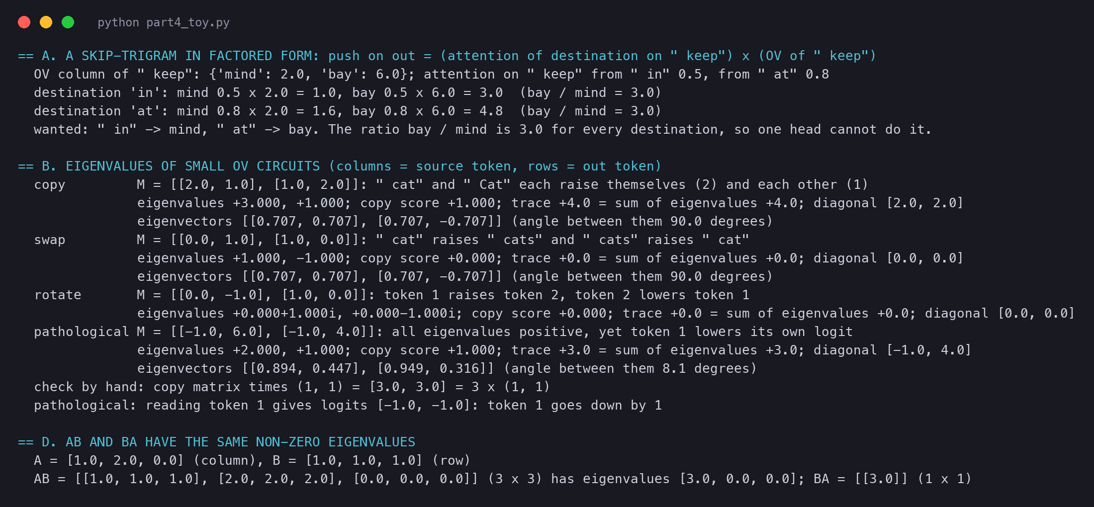
A tiny example. Let the OV column of " keep" raise " mind" by 2 and " bay" by 6. After " in", the head reads " keep" with weight 0.5. After " at", it reads " keep" with weight 0.8. Then:

Left: what the text needs. After "keep ... in", mind should be high and bay low; after "keep ... at", the other way round. Right: what one head gives with toy numbers. After "in": mind 0.5 × 2 = 1.0 and bay 0.5 × 6 = 3.0. After "at": mind 1.6 and bay 4.8. Bay is three times mind in both rows.

The head can change how loud it is, but not which idiom it prefers. If it is tuned for "keep at bay", it also says "bay" after "keep in".

On the real model. Our head 0.2 has exactly the paper's " keep" row. Here is its OV column for " keep" and its QK column for " keep":

plain text

== 5. A SKIP-TRIGRAM BUG: head 0.2 and " keep"
  OV column " keep": {' mind': 3.64, ' bay': 8.89, ' toes': 6.55, ' wraps': 2.71, ' forefront': 9.41}  (median over all tokens -0.09); top [' forefront', ' bay', '\n                   ', ' foreseeable', ' toes', ' slipping']
  QK column " keep": {' in': 1.78, ' at': 2.77, ' on': 1.74, ' under': 1.51, ' going': 3.58}  (median 0.12); top destinations [' looking', ' going', ' coming', ' searching', ' trying', ' happy']

The OV column is a list of idiom endings: "in the forefront", "at bay", "on your toes", "in mind", "under wraps". The typical entry is about zero, and these sit far above it. The QK column likes " in", " at", " on" and " under", and even more " going" and " looking" ("keep going", "keep looking").

Now the bug. We ran two prompts and measured what head 0.2 adds through the " keep" position alone:

plain text

  'You need to keep this in': head 0.2 puts 0.27 on " keep"; through " keep" it pushes mind +1.78, bay +5.28  (ratio bay/mind 2.96); whole head: mind +3.17, bay +4.76
      whole model: p(mind) = 0.6416, p(bay) = 0.000014; top 3 [' mind', ' the', ' your']; head 0.7 pushes mind +4.45
  'You need to keep the dogs at': head 0.2 puts 0.38 on " keep"; through " keep" it pushes mind +2.43, bay +7.19  (ratio bay/mind 2.96); whole head: mind +2.49, bay +7.49
      whole model: p(mind) = 0.0000, p(bay) = 0.318783; top 3 [' bay', ' the', ' home']; head 0.7 pushes mind +2.03

Head 0.2's push through the source " keep". In "You need to keep this in", it reads keep with weight 0.27 and pushes mind by 1.78 and bay by 5.28. In "You need to keep the dogs at", it reads keep with weight 0.38 and pushes mind by 2.43 and bay by 7.19. The ratio bay / mind is 2.96 in both prompts.

This is the factored form, measured. The ratio of the two pushes is 2.96 in both prompts, to two decimals. The destination changed the volume (0.27 or 0.38), but not the song. After "keep this in", head 0.2 raises the wrong idiom: " bay" by 5.28 and " mind" by only 1.78.

Yet the whole model gets it right: " mind" has probability 0.64 and " bay" only 0.000014. Other paths fix the bug. The bigram table knows that "in mind" is common and "in bay" is rare. Head 0.7 also pushes " mind" by 4.45. This is the "fungibility" warning in action: to judge one head, you must look at the rest of the model too.

The paper calls these bugs an early example of "using interpretability to understand model failures". The mistake was predicted from the shape of the weights, before running any text. Our run adds one detail: the bug is real in the head, but the rest of the model can hide it.

Making the tables smaller

Reading the largest entries works, but it is slow and selective. The paper asks for better summaries.

From the paperSummarizing OV/QK Matrices

What it says

The expanded matrices are "enormous, with easily billions of entries". Three reasons suggest that simpler summaries exist. They are "extremely low-rank": 50,000 × 50,000 but only rank $d_\text{head}$ . Entries hint at "cluster structure": in one head, names have top queries like " by" and places have top queries like " from". And "Copying behavior is widespread in OV matrices".

What it means

The first reason is the strongest. Part 2 showed that each 512 × 512 matrix of a head has rank 64. The 48,262 × 48,262 circuit is that matrix with the embedding and unembedding added on both sides, so its rank is still at most 64. A huge table that is really made of 64 directions should have a short description.

The second reason is about groups. If all names behave alike and all places behave alike, the table has blocks. Part 2 found the same in our head 0.3: on " in", it looked back at places; on " see", at first names.

Detecting copying with eigenvalues

From the paperDetecting Copying Behavior

What it says

Copying is "mapping the same vector to itself": a token raises its own probability. So it should fit some "summary statistic". But the right definition is hard to pin down. In slightly larger models, some heads copy "some mixture of gender, plurality, and tense". "So copying is actually a more complex concept than it might first appear."

What it means

A copying head is a mirror: what goes in comes back out. For a matrix, "comes back out" has an exact meaning in linear algebra. That is why the paper hopes for a clean test.

But think of a head that reads "she" and raises "her". Nothing is copied token by token. Still, the information "female" was copied. So the paper is careful: "copying" can mean the same token, a similar token, or the same property. Any one number will capture only some of these.

The exact meaning of "comes back out" is an eigenvector.

From the paperDetecting Copying Behavior

What it says

Take an OV circuit $M=W_{\mathrm{U}} W_{\mathrm{OV}}^h W_{\mathrm{E}}$ . An eigenvector with a positive eigenvalue is a combination of tokens "which increases the linear combination of logits of those same tokens". It is like a set of tokens which "mutually increase their own probability". A random matrix has an "equal number of positive and negative eigenvalues", and many complex ones. But "copying requires positive eigenvalues".

What it means

An OV circuit takes tokens in and gives logits out, and both sides are indexed by the same 48,262 tokens. So it is a square matrix, and "the same vector" makes sense on both sides. An eigenvector is a group of tokens. A positive eigenvalue says: read this group, and the head raises this same group.

The paper's examples of groups: all plural words, all words starting with one letter, or all spellings of one word (" Ralph", "Ralph", "RALPH"). An eigenvector can also have plus and minus parts, like "male words up, female words down". Then reading a male word raises male words and lowers female ones.

Random matrices have no reason to prefer positive eigenvalues. So if a head has almost only positive ones, training made it so, and copying is the natural reason.

A tiny example. Take a vocabulary of two tokens, " cat" and " Cat". A head reads one of them and raises it by 2, and the other one by 1. Its OV circuit is

M=\begin{bmatrix}2&1\\1&2\end{bmatrix}

Try the vector $v=(1,1)$ , "both spellings together". Then $Mv=(2+1,\;1+2)=(3,3)=3v$ . So $v$ is an eigenvector with eigenvalue 3. The other eigenvector is $(1,-1)$ with eigenvalue 1. Both eigenvalues are positive: this head copies.

Now a head that swaps: reading " cat" raises " cats", and reading " cats" raises " cat". Its matrix is $\begin{bmatrix}0&1\\1&0\end{bmatrix}$ , with eigenvalues $+1$ and $-1$ . The vector $(1,1)$ is kept, but $(1,-1)$ is flipped. This head does not copy; it moves between two tokens. A third head, $\begin{bmatrix}0&-1\\1&0\end{bmatrix}$ , raises token 2 when it reads token 1 and lowers token 1 when it reads token 2. Its eigenvalues are $+i$ and $-i$ , complex, because the matrix turns vectors instead of stretching them.

One number for each head

The paper collapses all the eigenvalues of a head into one number. Add up the eigenvalues, and divide by the sum of their sizes:

\text{copy score}=\frac{\sum_i\lambda_i}{\sum_i|\lambda_i|}

Read it this way. The bottom adds up the sizes of the eigenvalues. The top adds them with their signs, so positive and negative ones cancel, and complex pairs $x\pm iy$ lose their imaginary parts. If every eigenvalue is positive, top and bottom are equal and the score is 1. If every one is negative, the score is −1. A random mix gives about 0.

For our three small heads: the copying head has eigenvalues 3 and 1, so the score is $(3+1)/(3+1)=1$ . The swap head has $+1$ and $-1$ : $(1-1)/(1+1)=0$ . The rotating head has $+i$ and $-i$ : the top is 0, so the score is 0.

A trick to get the eigenvalues

A real OV circuit is 48,262 × 48,262. Finding all its eigenvalues directly would take a very long time. But the circuit is a product of a tall and a wide matrix, and a fact of linear algebra makes it small:

M=\underbrace{(W_{\mathrm{U}} W_{\mathrm{O}})}_{48{,}262\times64}\;\underbrace{(W_{\mathrm{V}} W_{\mathrm{E}})}_{64\times48{,}262},\qquad \text{non-zero eigenvalues of }PQ=\text{non-zero eigenvalues of }QP

Here $P=W_{\mathrm{U}} W_{\mathrm{O}}$ and $Q=W_{\mathrm{V}} W_{\mathrm{E}}$ . The product $QP$ is only 64 × 64. So the 48,262 × 48,262 circuit has 64 eigenvalues that matter, and all the others are zero.

A tiny example. Let $P=(1,2,0)$ as a column and $Q=(1,1,1)$ as a row. Then $PQ$ is a 3 × 3 matrix with rows $(1,1,1)$ , $(2,2,2)$ and $(0,0,0)$ . Its eigenvalues are 3, 0 and 0. And $QP=1+2+0=3$ , a 1 × 1 matrix with the single eigenvalue 3. The same non-zero eigenvalue, from a much smaller matrix.

On the real model. Our script checks the trick on a piece of head 0.0 small enough to do both ways: 300 tokens.

plain text

  check on a 300-token piece of head 0.0: 300 x 300 has 300 eigenvalues; the 64 largest match the 64 x 64 ones to 3.8e-13; the other 236 are at most 6.8e-14

The 64 large eigenvalues agree to 0.0000000000004, and the other 236 are zero up to rounding. So the 64 × 64 matrix gives the full answer.

What the paper found, and what we find

From the paperDetecting Copying Behavior

What it says

"10/12 of layer 1 heads have mostly positive OV eigenvalues, and appear to significantly perform copying". The plots use "a log scale to represent magnitude". For randomly initialised weights the eigenvalues spread over the whole disk, which is "very different from what we randomly expect".

What it means

Each small circle is one head. Each dot is one eigenvalue, placed by its direction: right means positive, left means negative, up and down mean complex. The distance from the centre is the size, on a log scale, because sizes range over many powers of ten.

The ten circled heads have nearly all their dots on the right. The two heads at the far left have dots everywhere. The random disk at the side is the baseline: no side is preferred. The contrast between the circled heads and the disk is the evidence.

We drew the same picture for our model, with one random head added for comparison:

The 64 non-zero eigenvalues of the OV circuit of each head of attn-only-1l, and of one random head. Dots on the right are positive. Heads 0.0, 0.3, 0.4, 0.6 and 0.7 have nearly all their dots on the right (copy scores +1.00, +1.00, +0.97, +0.91, +0.97); head 0.2 has most (+0.71); heads 0.1 and 0.5 lean left (−0.42, −0.37); the random head is spread evenly (about 0).

Here is our model, all eight heads:

plain text

  head 0.0: copy score sum(l)/sum(|l|) = +0.998; 64/64 with positive real part (26 real and positive, 38 complex); trace 353,117 = sum of diagonal 353,117
  head 0.1: copy score sum(l)/sum(|l|) = -0.418; 21/64 with positive real part (3 real and positive, 54 complex); trace -26,596 = sum of diagonal -26,596
  head 0.2: copy score sum(l)/sum(|l|) = +0.707; 42/64 with positive real part (14 real and positive, 46 complex); trace 93,844 = sum of diagonal 93,844
  head 0.3: copy score sum(l)/sum(|l|) = +1.000; 64/64 with positive real part (16 real and positive, 48 complex); trace 358,507 = sum of diagonal 358,507
  head 0.4: copy score sum(l)/sum(|l|) = +0.974; 61/64 with positive real part (19 real and positive, 44 complex); trace 235,602 = sum of diagonal 235,602
  head 0.5: copy score sum(l)/sum(|l|) = -0.365; 15/64 with positive real part (5 real and positive, 52 complex); trace -19,782 = sum of diagonal -19,782
  head 0.6: copy score sum(l)/sum(|l|) = +0.915; 61/64 with positive real part (13 real and positive, 50 complex); trace 155,782 = sum of diagonal 155,782
  head 0.7: copy score sum(l)/sum(|l|) = +0.970; 57/64 with positive real part (17 real and positive, 46 complex); trace 121,358 = sum of diagonal 121,358
  20 random Gaussian heads of the same shapes: copy score from -0.035 to +0.070 (mean -0.002); positive real part 29 to 35 of 64; complex 54 to 60 of 64

The copy score of every head of attn-only-1l: 0.0 +1.00, 0.3 +1.00, 0.4 +0.97, 0.7 +0.97, 0.6 +0.91, 0.2 +0.71, 0.5 −0.37, 0.1 −0.42. The thin dashed band around zero shows 20 random heads of the same shapes, from −0.035 to +0.070.

Six of our eight heads score above 0.7, and four score 0.97 or more. Twenty random heads of the same shapes all score between −0.035 and +0.070. Training clearly pushed most heads towards copying, as in the paper's model.

The two heads with negative scores, 0.1 and 0.5, are two of the positional heads from earlier. They do not copy: they look one token back and predict what comes next, like "couldn" → "t". This matches the paper's picture, where most heads copy and a few do something else.

Where the score can fool you

From the paperDetecting Copying Behavior

What it says

Copying matrices must have positive eigenvalues, but the reverse is not certain. "A matrix's eigenvectors aren't necessarily orthogonal". So a matrix with all positive eigenvalues can "map some tokens to decreasing the logits of that same token". Positive eigenvalues mean "copying on average". They are strong evidence, but not a "dispositive proof" (a final proof).

What it means

Eigenvectors at right angles behave nicely: each token splits cleanly into eigenvector parts. Eigenvectors at a narrow angle do not. Then a token can be a big plus of one eigenvector and a big minus of another, and the stretches can work against each other.

So a score of 1 says the head copies groups of tokens on average. It does not promise that every single token is copied.

A tiny example. Take this OV circuit of two tokens:

M=\begin{bmatrix}-1&6\\-1&4\end{bmatrix}

Its eigenvalues are 2 and 1, both positive, so its copy score is 1. You can check one: $M\,(2,1)=(-2+6,\;-2+4)=(4,2)=2\,(2,1)$ . But look at the first column: reading token 1 gives the logits $(-1,-1)$ . Token 1 lowers its own logit. The two eigenvectors, $(2,1)$ and $(3,1)$ , point almost the same way: the angle between them is only 8.1 degrees. That narrow angle is what lets the matrix "copy on average" while one token does the opposite.

Other ways to measure copying

From the paperDetecting Copying Behavior

What it says

One could also "look at the diagonal": how each token changes its own probability. Or ask how often a token raises itself more than any other token, or is among the top $k$ . All these measures are linked, because "the sum of the eigenvalues is equal to the trace is equal to the sum of the diagonal". The paper keeps the "eigenvalue-based summary statistic".

What it means

The diagonal entry $M_{t,t}$ answers the simplest question: if the head reads token $t$ , does $t$ go up? The top-1 test is stricter: is $t$ the token that goes up most?

The link is a classic fact of linear algebra. The trace of a matrix, the sum of its diagonal, always equals the sum of its eigenvalues. So the top of the copy score is just the sum of all "does $t$ raise itself?" numbers. The measures look at the same matrix from different sides.

The fact is easy to check. For our copying toy, the diagonal is $(2,2)$ with sum 4, and the eigenvalues are 3 and 1, also sum 4. For the pathological toy, $-1+4=3=2+1$ . For the real heads, the printout above shows the trace of the 64 × 64 matrix. Next to it is the sum of all 48,262 diagonal entries of the full circuit. They agree in every head: for head 0.0, both are 353,117.

Our script also computed the other measures:

Head	Copy score	Diagonal > 0	Top-1 self	Top-5 self
0.0	+0.998	0.99	0.37	0.51
0.1	−0.418	0.37	0.00	0.00
0.2	+0.707	0.91	0.00	0.01
0.3	+1.000	0.98	0.34	0.43
0.4	+0.974	0.96	0.26	0.34
0.5	−0.365	0.38	0.00	0.00
0.6	+0.915	0.92	0.12	0.21
0.7	+0.970	0.96	0.00	0.02

"Diagonal > 0" is the share of all 48,262 tokens that raise their own logit. "Top-1 self" and "top-5 self" use tokens 1,000 to 2,999. They ask: is the token itself the first, or among the first five, tokens it raises?

Most measures agree, but look at head 0.7. Its copy score is 0.97, and 96% of tokens raise themselves. Yet a token is almost never its own top output: top-1 is 0.00. Earlier we saw why: on " Paris", head 0.7 raises Frankfurt, Amsterdam and Milan, not Paris. It copies the kind of token, "a city", not the token. This is exactly the paper's warning that copying "is actually a more complex concept than it might first appear".

Do we understand one-layer models?

The paper ends its study of one-layer models with an honest question.

From the paperDo We "Fully Understand" One-Layer Models?

What it says

We understand the one-layer model the way "one might look at the weights of a giant linear regression" or a large database. "There's no longer any algorithmic mystery." But "there's far too much there for one to hold the model in their head". Since one-layer networks are generalized linear models, perhaps it is not surprising that "a single attention layer is mostly one as well".

What it means

Think of a phone book. You understand completely how it works: find the name, read the number. There is no mystery. But you do not know all the numbers in it, and you could not recite them.

That is where one-layer models stand after this part. We know the mechanism exactly: look back with the QK table, change the logits with the OV table. We can predict its bugs from that mechanism. But the tables hold 37.3 billion numbers, and no one can keep them in mind.

The last sentence lowers the drama on purpose. A regression is a weighted sum of inputs. A one-layer attention model, with the pattern held fixed, is a weighted sum of skip-trigram tables. The surprising things begin with two layers, where heads can work together. That is Part 5.

Key takeaways

Every head has two tables. The QK circuit ${W_{\mathrm{E}}}^{\top} W_{\mathrm{QK}}^h W_{\mathrm{E}}$ says which earlier tokens a destination reads. The OV circuit $W_{\mathrm{U}} W_{\mathrm{OV}}^h W_{\mathrm{E}}$ says what reading a token does to the logits. Once a destination has chosen how much to read a source, the effect depends only on the source.
Together they store skip-trigrams, "[source] ... [destination] → [out]". In attn-only-1l, head 0.0 at "R" reads " Ralph" with weight 0.59 and raises "alph" by 8.18. With "Ralph" earlier, the model gives "alph" 0.83; with "Bob", 0.02.
The tables are huge. Our model stores 51.0 million weights, but its expanded QK and OV circuits hold 37.3 billion numbers: readable cards, but far too many to read.
Most heads copy. Their OV circuits raise the token they read, or similar tokens; their QK circuits read only tokens that fit next. This is a very primitive in-context learning.
Some heads are positional. From positions alone, heads 0.1, 0.5 and 0.7 put 0.88 to 0.94 on the current token and the rest on the previous one. Head 0.5 reads " corresponding" and raises " to", as in the paper.
The factored form makes bugs. A head that raises "keep ... in mind" and "keep ... at bay" must also raise "keep ... in bay". Our head 0.2 pushes " bay" 2.96 times more than " mind" after both "keep this in" and "keep the dogs at". Other paths hide the bug in the full model.
Eigenvalues detect copying. A positive eigenvalue of an OV circuit means a group of tokens that raises itself. The copy score $\sum\lambda_i/\sum|\lambda_i|$ is above 0.7 for six of our eight heads, against −0.035 to +0.070 for random heads. The paper found 10 of 12.
Copying has many meanings. Trace = sum of eigenvalues = sum of the diagonal links the measures, but they can disagree. Head 0.7 scores 0.97, yet a token is almost never its own top output: it copies "a city", not "Paris".
One-layer models are understood like a database: no mystery in the mechanism, too much content to hold in mind.

Next, in Part 5: a second layer lets heads read what earlier heads wrote. The paper calls this composition and finds three kinds of it: Q-, K- and V-composition. Part 6 then shows the circuit that composition makes possible, the induction head, the stronger form of in-context learning promised in this part.

Run it yourself

The two scripts behind this part are circuits_part4.py (every real-model number: the size of the circuits, the skip-trigram tables, the prompts, the positional heads, the "keep" bug, the 64 × 64 trick, the eigenvalues and the other copying measures) and circuits_part4_toy.py (the hand-sized examples). They use TransformerLens 3.x and attn-only-1l on the CPU. The positional measurement reads 1,000 tokens of part1.md, so its numbers move a little if that page changes.

bash

pip install torch "transformer_lens<4"
python circuits_part4.py        # writes results/part4.json and results/part4_stdout.txt
python circuits_part4_toy.py    # writes results/part4_toy.json

Terminal output of circuits_part4.py: the size of the circuits, the skip-trigram tables of heads 0.0, 0.6 and 0.7, the prompts with Ralph and perfect, the positional heads, the keep bug of head 0.2, the 64 by 64 eigenvalue trick, and the copy score of every head — The real output of circuits_part4.py.

Terminal output of circuits_part4_toy.py: the factored keep example, the eigenvalues of the copy, swap, rotation and pathological matrices, and AB versus BA — The real output of circuits_part4_toy.py.

The paper and the code

A Mathematical Framework for Transformer Circuits (Transformer Circuits Thread, 2021) · our scripts for this part

One-Layer Models: Skip-Trigrams, Copying and Their Bugs

The two circuits of every head#

Skip-trigrams#

A giant pile of cards#

Copying#

Copying words that are split in two#

A very simple kind of in-context learning#

Not only copying#

Heads that look at position#

Skip-trigram bugs#

Making the tables smaller#

Detecting copying with eigenvalues#

One number for each head#

A trick to get the eigenvalues#

What the paper found, and what we find#

Where the score can fool you#

Other ways to measure copying#

Do we understand one-layer models?#

The paper and the code#

The two circuits of every head

Skip-trigrams

A giant pile of cards

Copying

Copying words that are split in two

A very simple kind of in-context learning

Not only copying

Heads that look at position

Skip-trigram bugs

Making the tables smaller

Detecting copying with eigenvalues

One number for each head

A trick to get the eigenvalues

What the paper found, and what we find

Where the score can fool you

Other ways to measure copying

Do we understand one-layer models?

The paper and the code