Circuits, explained · Part 3 of 7 · Covers Conceptual take-aways, One-Layer Attention-Only Transformers, The Path Expansion Trick, OV and QK Independence, Path Expansion of Logits

Paths Through the Model: the Path Expansion Trick

How the paper turns a one-layer model into a sum of end-to-end paths, one for the token itself and one for each head. We expand the real model, freeze its attention, and check every term.

A Mathematical Framework for Transformer Circuits. Nelson Elhage, Neel Nanda, Catherine Olsson, Tom Henighan, Nicholas Joseph, Ben Mann, Amanda Askell, Yuntao Bai, Anna Chen, Tom Conerly, Nova DasSarma, Dawn Drain, Deep Ganguli, Zac Hatfield-Dodds, Danny Hernandez, Andy Jones, Jackson Kernion, Liane Lovitt, Kamal Ndousse, Dario Amodei, Tom Brown, Jack Clark, Jared Kaplan, Sam McCandlish, Chris Olah. Transformer Circuits Thread, 2021.

Parts 1 and 2 took the model apart piece by piece: the residual stream, then one attention head. This part puts the pieces back together in a new shape: a sum of paths from the input tokens to the output. Every path can be read on its own.

We use the same one-layer model, attn-only-1l, and the same prompt as Part 2: "I like green tea, so I drink green". The model's next word is " tea", with probability 0.897. By the end of this part we will know exactly how much each path adds to that guess.

The promise: a sum of simple functions

The paper states its main method early, in a short list of "conceptual take-aways". Two items of that list are the subject of this part.

From the paperSummary of Results

What it says

"Attention-only models can be written as a sum of interpretable end-to-end functions mapping tokens to changes in logits." These functions "correspond to 'paths' through the model, and are linear if one freezes the attention patterns." Also: "Transformers have an enormous amount of linear structure", and one can learn a lot "by breaking apart sums and multiplying together chains of matrices".

What it means

Think of a big river delta. Water from the mountain reaches the sea along many channels. You cannot see much by looking at the whole delta at once. But you can follow one channel from the source to the sea, measure its flow, and then add up the channels.

The paper says that a small transformer is like that delta. The tokens are the source, and the logits are the sea. Each "path" is one channel through the layers. Each path is an "end-to-end function": it starts at the tokens and ends at the logits, so a person can read it in tokens.

The second sentence names the tool. Most of a transformer is matrix multiplication and addition. Only the attention pattern is not. So if we hold the attention pattern fixed, everything left is linear algebra, and linear algebra can be taken apart. This part shows how.

The two words "freezes" and "linear" carry the whole idea. We meet both again below, and we test them on the real model.

One layer: a bigram model plus skip-trigrams

The section on one-layer models opens with a claim, and then says what it will do with it.

From the paperOne-Layer Attention-Only Transformers

What it says

A one-layer attention-only transformer is "an ensemble of a bigram model and several 'skip-trigram' models". They change the probabilities of sequences "A… BC". Each head can "selectively attend from the present token ('B') to a previous token ('A')". It copies information that changes the probability of the next token ("C"). The goal is to "convert the raw weights of a transformer into interpretable tables".

What it means

Think of a panel of judges who each give a score, and the scores are added. One judge only looks at the current word. That is the bigram model from Part 1: "after Barack, say Obama". Each other judge is a head. A head looks back at one earlier word and then votes for some next words.

The phrase "A… BC" is the pattern a head can learn. "A" is an earlier token, "B" is the current token, and "C" is the next token. The dots mean that any number of tokens can sit between A and B. In our prompt, A is " tea", B is the last " green", and C is " tea" again.

The last sentence is the real promise. The paper does not only want to describe the model. It wants tables that you can read straight from the weights, without running any text. This part builds the sum that holds those tables, and Part 4 reads them.

"Ensemble" is a strong word. It says that the one-layer model is nothing more than its members, added together. To check this, we need to write the model in a form where the sum is visible. That form is the path expansion.

The model as a product

Before the trick, the paper writes the one-layer model again, in three lines.

From the paperThe Path Expansion Trick

What it says

A one-layer attention-only transformer is "a token embedding, followed by an attention layer" and "finally an unembedding". In equations: $x_0=W_{\mathrm{E}}\,t$ , then $x_1=x_0+\sum_{h\in H}h(x_0)$ , then $T(t)=W_{\mathrm{U}}\,x_1$ . With the tensor notation of Part 2, the model is "a product of three terms".

What it means

Read the figure from the bottom up, like the model runs. The tokens become vectors. Every head reads those vectors and adds its output. The unembedding turns the result into logits. These are the equations of Part 1, with only one layer.

The plus sign in the middle is important. The heads do not replace the stream; they add to it. The original $x_0$ is still there in $x_1$ . This is the residual stream at work, and it is the reason the expansion below gives more than one path.

"A product of three terms" means one factor for each stage: embed, attend, unembed. The next figure of the paper writes the three factors out.

Here $t$ is the whole prompt as one table of one-hot vectors, one column per position. So $x_0$ and $x_1$ are tables too, with one stream vector per position. Each head works on the whole table, because it reads across positions.

From the paperThe Path Expansion Trick

What it says

$T=(\text{Id}\otimes W_{\mathrm{U}})\cdot\big(\text{Id}+\sum_{h\in H_1}A^h\otimes W_{\mathrm{OV}}^h\big)\cdot(\text{Id}\otimes W_{\mathrm{E}})$ . The unembedding "maps residual stream vectors to logits". The attention layer adds the result of each head. The embedding "maps tokens to residual stream vectors". The pattern is $A^h=\text{softmax}^*(t^\top W_{\mathrm{E}}^\top W_{\mathrm{QK}}^h W_{\mathrm{E}}\,t)$ .

What it means

Each factor is one stage of the figure above, written as a map from tables to tables. The right factor embeds every token. The middle factor runs the attention layer. The left factor unembeds every position. A product of maps means "do the right one first, then the next".

The notation comes from Part 2. $\text{Id}\otimes W$ means "apply $W$ to each position, and do not mix positions". $A^h\otimes W_{\mathrm{OV}}^h$ is one whole head: the pattern mixes positions, and $W_{\mathrm{OV}}^h$ changes each vector. The lone $\text{Id}$ in the middle is the plus sign of the residual stream: "keep what was there".

The second line says where the pattern comes from. It is the masked softmax of scores, and each score multiplies two tokens through $W_{\mathrm{E}}^\top W_{\mathrm{QK}}^h W_{\mathrm{E}}$ . That is the QK circuit of Part 2. So the pattern depends on the tokens too, which is the only non-linear part of the model.

Check the product on the real model

Is this product really the model? We computed it by hand, stage by stage, at all ten positions of our prompt:

python

x0  = E + P                                                     # (Id ⊗ W_E) t, plus the position embedding
mid = x0 + sum(A[h] @ (x0 / s1[:, None]) @ OV[h] for h in range(8)) + bias_O   # (Id + Σ_h A^h ⊗ W_OV^h) x0
prod = (mid / sf[:, None]) @ W_U + b_U                          # (Id ⊗ W_U) x1

plain text

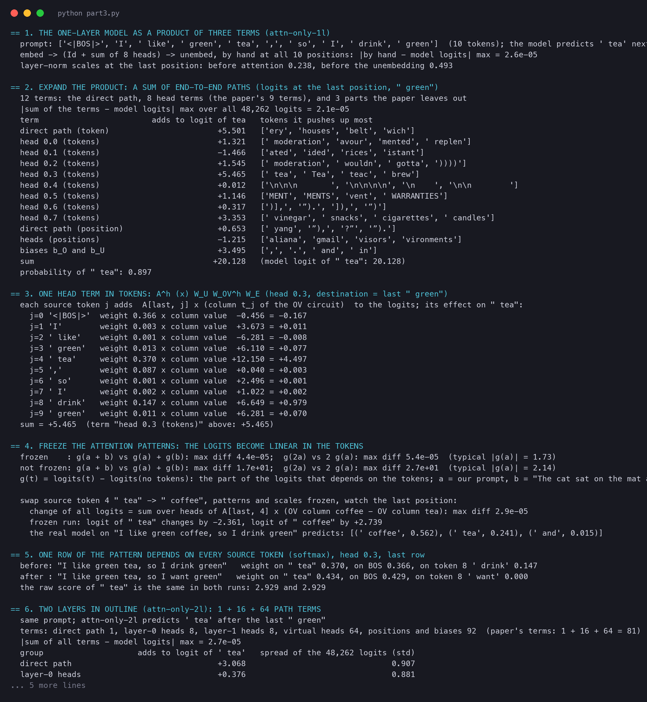
== 1. THE ONE-LAYER MODEL AS A PRODUCT OF THREE TERMS (attn-only-1l)
  prompt: ['<|BOS|>', 'I', ' like', ' green', ' tea', ',', ' so', ' I', ' drink', ' green']  (10 tokens); the model predicts ' tea' next
  embed -> (Id + sum of 8 heads) -> unembed, by hand at all 10 positions: |by hand - model logits| max = 2.6e-05
  layer-norm scales at the last position: before attention 0.238, before the unembedding 0.493

The largest difference over all 48,262 logits at all ten positions is 0.000026, which is rounding noise. Three things in the code are not in the paper's formula. The real model adds a position embedding P to each token's vector. It has biases (bias_O, b_U). And it has the leftover layer norm from Part 1, which divides each vector by a scale (s1, sf).

We read the layer-norm scales from the real run and then hold them fixed. With fixed scales, a division is just a multiplication by a number, so it fits inside the product. The scales at the last position are 0.238 and 0.493. The paper's models have no layer norm, so it does not need this step.

Expand the product

Now comes the trick. It is the oldest move in algebra: multiply out the brackets.

Take a product of two sums of numbers, $(1+2)\times(1+3)$ . You can add first and then multiply: $3\times4=12$ . Or you can multiply every part of the first bracket by every part of the second and add the results: $1+2+3+2\times3=12$ . The answer is the same. The second way keeps a record of where each part of the answer came from.

From the paperThe Path Expansion Trick

What it says

"Our key trick is to simply expand the product." This turns a product, "where every term corresponds to a layer", into "a sum where every term corresponds to an end-to-end path": $T=\text{Id}\otimes W_{\mathrm{U}} W_{\mathrm{E}}+\sum_{h\in H}A^h\otimes(W_{\mathrm{U}} W_{\mathrm{OV}}^h W_{\mathrm{E}})$ . Each term is "tractable to understand, can be reasoned about independently, and additively combine[s] to create model behavior".

What it means

Before the trick, the model is a pipeline: every token passes through every stage. After the trick, it is a set of separate routes. The direct path goes from the token straight to the logits. Each head term goes from the tokens, through one head, to the logits.

The key change is in what each piece means. A layer is hard to read, because its input and output are 512-number vectors. A path starts at tokens and ends at logits, so it is a table from tokens to tokens. A person can read that.

The last claim has three parts, and this part tests each one. "Tractable": each term is a product of known matrices. "Independently": we can compute one term without the others. "Additively": the terms add up to the model, as the check below shows.

The derivation

The middle factor is a sum of nine parts: $\text{Id}$ and one term per head. The outer factors have one part each. So the expansion has $1\times9\times1=9$ products. Take the first one, with $\text{Id}$ from the middle:

\begin{aligned} &(\text{Id}\otimes W_{\mathrm{U}})\cdot\text{Id}\cdot(\text{Id}\otimes W_{\mathrm{E}})\\ &=(\text{Id}\cdot\text{Id})\otimes(W_{\mathrm{U}} W_{\mathrm{E}})\\ &=\text{Id}\otimes W_{\mathrm{U}} W_{\mathrm{E}} \end{aligned}

The middle $\text{Id}$ changes nothing, so it disappears. The second line is the mixed-product property from Part 2: $(A\otimes B)(C\otimes D)=(AC)\otimes(BD)$ . The left sides of the two factors multiply, and the right sides multiply. Now take one head $h$ from the middle:

\begin{aligned} &(\text{Id}\otimes W_{\mathrm{U}})(A^h\otimes W_{\mathrm{OV}}^h)(\text{Id}\otimes W_{\mathrm{E}})\\ &=(\text{Id}\,A^h\,\text{Id})\otimes(W_{\mathrm{U}} W_{\mathrm{OV}}^h W_{\mathrm{E}})\\ &=A^h\otimes W_{\mathrm{U}} W_{\mathrm{OV}}^h W_{\mathrm{E}} \end{aligned}

The same rule puts everything that acts on positions on the left of $\otimes$ and everything that acts on vectors on the right. On the left, only the pattern $A^h$ is left. On the right, the chain of matrices runs from the token to the logits. Add the nine products, and you get the paper's sum.

Read each symbol once more. $\text{Id}\otimes W_{\mathrm{U}} W_{\mathrm{E}}$ is the direct path: no mixing of positions, and the table $W_{\mathrm{U}} W_{\mathrm{E}}$ from Part 1. $A^h\otimes W_{\mathrm{U}} W_{\mathrm{OV}}^h W_{\mathrm{E}}$ is the head term of head $h$ . The pattern $A^h$ says which positions are read. The table $W_{\mathrm{U}} W_{\mathrm{OV}}^h W_{\mathrm{E}}$ says what reading each token does to the logits. That table is the OV circuit of Part 2.

A toy you can check by hand

Our toy model has three tokens, a, b and c, a stream of 2 numbers and one head. The embedding puts a at $(1,0)$ , b at $(0,1)$ and c at $(1,1)$ . The unembedding reads the logit of a from number 1 and the logit of b from number 2, and c always gets 0. The head swaps the two numbers. On the text "a b", position 2 reads both tokens, half each.

The toy model on the text "a b", at position 2. Left, the product, layer after layer: the embedding gives (0, 1), the head adds (0.5, 0.5), so the stream is (0.5, 1.5), and the unembedding gives the logits (0.5, 1.5, 0). Right, the sum of paths: the direct path gives (0, 1, 0) and the head term gives (0.5, 0.5, 0). Their sum is the same (0.5, 1.5, 0).

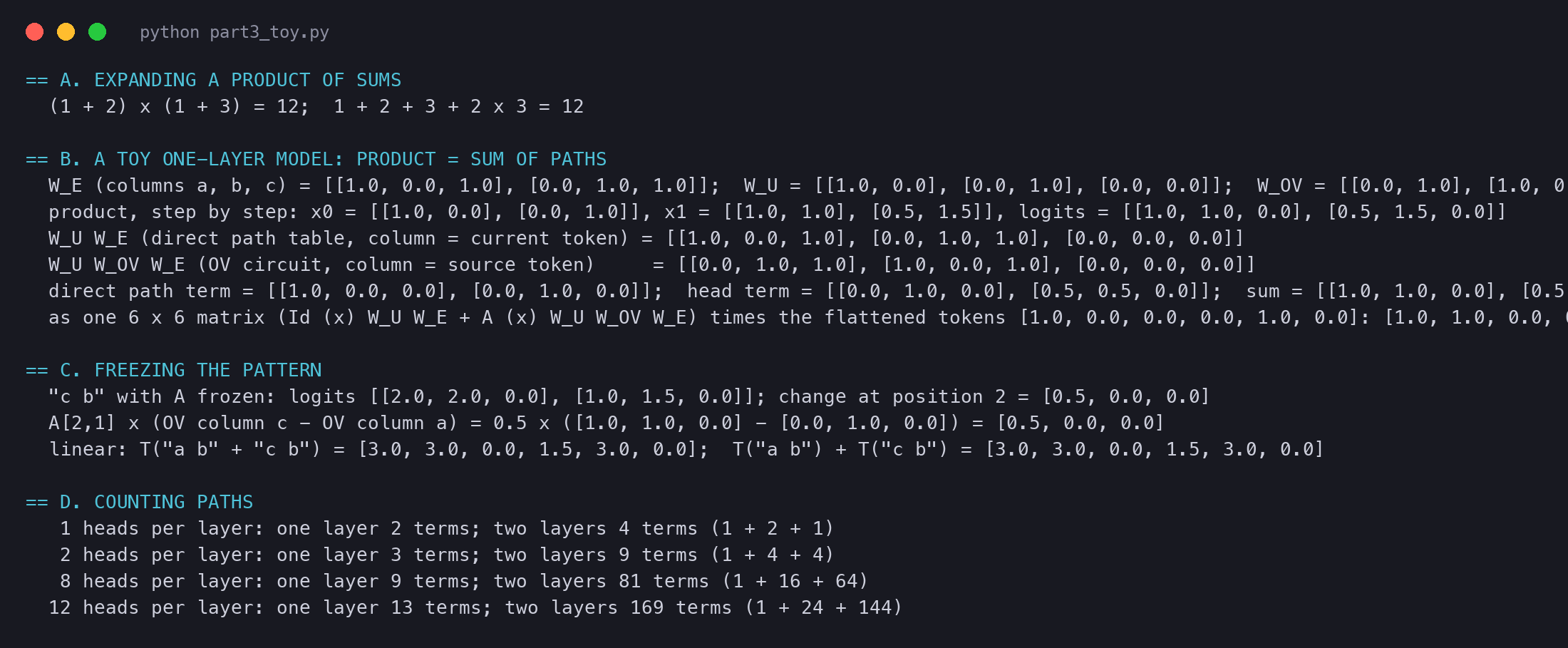
Work the head term out by hand. The OV table $W_{\mathrm{U}} W_{\mathrm{OV}} W_{\mathrm{E}}$ has one column per source token. Reading a gives $(0,1,0)$ , because the head swaps $(1,0)$ to $(0,1)$ , which is the logit of b. Reading b gives $(1,0,0)$ . Position 2 takes half of each column: $0.5\times(0,1,0)+0.5\times(1,0,0)=(0.5,0.5,0)$ . The script prints the same numbers:

plain text

  W_U W_OV W_E (OV circuit, column = source token)     = [[0.0, 1.0, 1.0], [1.0, 0.0, 1.0], [0.0, 0.0, 0.0]]
  direct path term = [[1.0, 0.0, 0.0], [0.0, 1.0, 0.0]];  head term = [[0.0, 1.0, 0.0], [0.5, 0.5, 0.0]];  sum = [[1.0, 1.0, 0.0], [0.5, 1.5, 0.0]]
  as one 6 x 6 matrix (Id (x) W_U W_E + A (x) W_U W_OV W_E) times the flattened tokens [1.0, 0.0, 0.0, 0.0, 1.0, 0.0]: [1.0, 1.0, 0.0, 0.5, 1.5, 0.0]

The last line writes the whole toy model, with $A$ fixed, as one 6 × 6 matrix. It acts on the two one-hot tokens laid end to end. With $A$ fixed, the model really is one matrix times the tokens.

The paths of the real model

Now the real model. At the last position, the one that predicts " tea", we computed every path term over all 48,262 logits. Each head term is computed in tokens, as the formula says: the pattern of the head times the token columns of its OV table.

python

terms['direct path (token)'] = (E[i] / sf[i]) @ W_U                                     # Id ⊗ W_U W_E
for h in range(8):
    terms[f'head 0.{h} (tokens)'] = (A[h, i] @ (E / s1[:, None]) @ OV[h] / sf[i]) @ W_U   # A^h ⊗ W_U W_OV^h W_E

plain text

== 2. EXPAND THE PRODUCT: A SUM OF END-TO-END PATHS (logits at the last position, " green")
  12 terms: the direct path, 8 head terms (the paper's 9 terms), and 3 parts the paper leaves out
  |sum of the terms - model logits| max over all 48,262 logits = 2.1e-05
  term                        adds to logit of tea   tokens it pushes up most
  direct path (token)                       +5.501   ['ery', 'houses', 'belt', 'wich']
  head 0.0 (tokens)                         +1.321   [' moderation', 'avour', 'mented', ' replen']
  head 0.1 (tokens)                         -1.466   ['ated', 'ided', 'rices', 'istant']
  head 0.2 (tokens)                         +1.545   [' moderation', ' wouldn', ' gotta', '))))']
  head 0.3 (tokens)                         +5.465   [' tea', ' Tea', ' teac', ' brew']
  head 0.4 (tokens)                         +0.012   ['\n\n\n       ', '\n\n\n\n', '\n    ', '\n\n        ']
  head 0.5 (tokens)                         +1.146   ['MENT', 'MENTS', 'vent', ' WARRANTIES']
  head 0.6 (tokens)                         +0.317   [')],', '”).', ']),', '”)']
  head 0.7 (tokens)                         +3.353   [' vinegar', ' snacks', ' cigarettes', ' candles']
  direct path (position)                    +0.653   [' yang', '”),', '?”', '”).']
  heads (positions)                         -1.215   ['aliana', 'gmail', 'visors', 'vironments']
  biases b_O and b_U                        +3.495   [',', '.', ' and', ' in']
  sum                                      +20.128   (model logit of " tea": 20.128)

How much each path of attn-only-1l adds to the logit of "tea" at the last "green". The direct path adds +5.501 and head 0.3 adds +5.465; head 0.7 adds +3.353 and the biases +3.495; head 0.1 takes away 1.466. The first nine rows are the paper's terms, and all twelve add up to 20.128, the model's real logit.

The twelve terms add up to the model's logits. The largest error over all 48,262 logits is 0.000021. So the expansion is not an approximation. It is the model, written another way.

Now the table can be read. Two paths carry most of the vote for " tea". The direct path adds +5.501, and head 0.3 adds +5.465. Head 0.7 adds +3.353, and head 0.1 votes against with −1.466. The other heads add a little.

The last three rows are parts the paper leaves out: the position embedding, through the direct path and through the heads, and the biases. They do not depend on which tokens are in the prompt, only on where they are. That is why the paper can drop them and still describe what the model does with tokens.

The direct path

From the paperThe Path Expansion Trick

What it says

The direct path term, $\text{Id}\otimes W_{\mathrm{U}} W_{\mathrm{E}}$ , "also occurred when we looked at the zero-layer transformer". "Because it doesn't move information between positions", "the only thing it can contribute to is the bigram statistics". It will "fill in missing gaps that other terms don't handle".

What it means

The $\text{Id}$ on the left of $\otimes$ says it all. The direct path at position $i$ only sees the token at position $i$ . It is the zero-layer model of Part 1, still sitting inside the one-layer model.

A path that sees one token can only store "after this token, that token is likely". So it can only hold bigrams. And because the heads also predict some bigrams, the direct path does not hold the full bigram table. It holds what is left: the bigrams that the heads do not already cover.

This is how the terms share work. No term is told what to do. Training shapes all of them together, and each one ends up with the part of the job that suits its shape.

Look at the top tokens of the direct path at the last " green": "ery", "houses", "belt" and "wich". These pieces complete "greenery", "greenhouses", "greenbelt" and "Greenwich". That is bigram knowledge in its purest form: it only needs the current token.

But the direct path also adds +5.501 to " tea". "Green tea" is a common phrase, so " tea" after " green" is a good bigram too. Without the head, this is the only reason the model would think of tea. The head adds a second, separate reason: "tea" appeared earlier in this text.

The head terms

The section after the trick starts from one head term and asks what it means.

From the paperSplitting Attention Head terms into Query-Key and Output-Value Circuits

What it says

"For each attention head $h$ we have a term $A^h\otimes(W_{\mathrm{U}} W_{\mathrm{OV}}^h W_{\mathrm{E}})$ where $A^h=\text{softmax}(t^\top\cdot W_{\mathrm{E}}^\top W_{\mathrm{QK}}^h W_{\mathrm{E}}\cdot t)$ ." Then two questions: "How can we map these terms to model behavior?" and "why do we get these particular products of matrices on our equations?"

What it means

The head term has two halves, and each half comes from a chain of matrices. Both chains begin with $W_{\mathrm{E}}$ , because both begin at tokens. The OV chain ends with $W_{\mathrm{U}}$ , because it ends at logits. The QK chain ends with a token on each side, because a score compares two tokens.

That is the answer to "why these products". Each product is a path traced through the model, from where the information enters to where it is used. Part 2 named the two tables: the QK circuit and the OV circuit.

The first question, about behaviour, is what Part 4 answers with skip-trigrams. Here we do one smaller step: we take one real head term apart into its tokens.

What does $A^h\otimes W_{\mathrm{U}} W_{\mathrm{OV}}^h W_{\mathrm{E}}$ do at one position $i$ ? Apply it to the prompt $t$ , and read row $i$ . The result is a sum over the source positions $j$ :

\big[(A^h\otimes W_{\mathrm{U}} W_{\mathrm{OV}}^h W_{\mathrm{E}})\,t\big]_i=\sum_{j\le i}A^h_{ij}\,\big(W_{\mathrm{U}} W_{\mathrm{OV}}^h W_{\mathrm{E}}\big)\,t_j

Read it left to right. The head term at position $i$ is a weighted sum. Each source position $j$ gives one column of the OV table: the column of its own token $t_j$ . The weight of that column is $A^h_{ij}$ , how much position $i$ reads position $j$ .

In the toy, position 2 had weights 0.5 and 0.5 on a and b. So its head term was half of column a plus half of column b. On the real model, here is head 0.3 at the last " green", for the logit of " tea":

plain text

== 3. ONE HEAD TERM IN TOKENS: A^h (x) W_U W_OV^h W_E (head 0.3, destination = last " green")
  each source token j adds  A[last, j] x (column t_j of the OV circuit)  to the logits; its effect on " tea":
    j=0 '<|BOS|>'  weight 0.366 x column value  -0.456 = -0.167
    j=1 'I'        weight 0.003 x column value  +3.673 = +0.011
    j=2 ' like'    weight 0.001 x column value  -6.281 = -0.008
    j=3 ' green'   weight 0.013 x column value  +6.110 = +0.077
    j=4 ' tea'     weight 0.370 x column value +12.150 = +4.497
    j=5 ','        weight 0.087 x column value  +0.040 = +0.003
    j=6 ' so'      weight 0.001 x column value  +2.496 = +0.001
    j=7 ' I'       weight 0.002 x column value  +1.022 = +0.002
    j=8 ' drink'   weight 0.147 x column value  +6.649 = +0.979
    j=9 ' green'   weight 0.011 x column value  +6.281 = +0.070
  sum = +5.465  (term "head 0.3 (tokens)" above: +5.465)

Head 0.3 at the last "green", taken apart by source token. For each token: the attention weight, the value of that token's OV column in the row for "tea", and their product. "Tea" has weight 0.370 and column value +12.15, so it adds +4.497. "Drink" adds +0.979 and BOS takes away 0.167. The total, +5.465, is the head 0.3 term.

Almost all of the head's vote comes from one source: " tea" at position 4. Its column has the value +12.15 in the row for " tea", the largest of all ten sources. That is the copying behaviour of Part 2: reading " tea" pushes up " tea". The weight 0.370 decides how much of that column arrives.

The two rows for " green" have different column values, +6.110 and +6.281. The token is the same, but the layer-norm scales of the two positions differ a little, because their position embeddings differ. Our columns include the scales. In the paper's model, with no layer norm, the two columns would be equal.

Where and what, once more

The paper then explains why the two halves of the head term can be thought about apart.

From the paperSplitting Attention Head terms into Query-Key and Output-Value Circuits

What it says

The attention pattern depends on both the source and the destination token. But once the weight is set, the effect on the output "is solely a function of that source token". If several destinations read the same source by the same amount, "the source token will have the same effect on the logits". A footnote adds that, technically, the pattern depends on "all possible source tokens from the start to the destination token", because the softmax normalises.

What it means

Think of a radio. The volume knob depends on who is listening and what they want. But the song on the station does not depend on the listener. Two people with the knob at the same level hear exactly the same song.

In the head, the knob is the weight $A^h_{ij}$ , and the song is the OV column of the source token. Look at the formula above: the column $(W_{\mathrm{U}} W_{\mathrm{OV}}^h W_{\mathrm{E}})\,t_j$ contains only $t_j$ . Nothing about position $i$ enters it. Only the weight knows about the destination.

The footnote is a fair warning. The weight on one source is not decided by that source alone. The softmax divides by a sum over all sources, so a change anywhere in the row moves every weight. We test this next.

We changed one token of the prompt, " drink", to " want", and looked at the last row of head 0.3 again:

plain text

== 5. ONE ROW OF THE PATTERN DEPENDS ON EVERY SOURCE TOKEN (softmax), head 0.3, last row
  before: "I like green tea, so I drink green"   weight on " tea" 0.370, on BOS 0.366, on token 8 ' drink' 0.147
  after : "I like green tea, so I want green"   weight on " tea" 0.434, on BOS 0.429, on token 8 ' want' 0.000
  the raw score of " tea" is the same in both runs: 2.929 and 2.929

The last row of head 0.3's pattern, before and after one token changes. Before, BOS and "tea" each get about 0.37 and "drink" gets 0.15. After "drink" becomes "want", the head gives "want" no weight, and BOS and "tea" rise to 0.43 each. The score of "tea" did not change, but the softmax shares out the weight that "want" left free.

The score between the last " green" and " tea" did not change: 2.929 in both runs. Only the token at position 8 changed. Yet the weight on " tea" rose from 0.370 to 0.434. The new token " want" took no weight, and the softmax gave its share to the others. This is what the footnote means: the QK circuit gives each pair a score, but the weight of a pair depends on the whole row.

Freezing the attention patterns

The head term has one non-linear piece: the pattern $A^h$ , which comes from a softmax of the tokens. The paper now offers a way to remove even that.

From the paperOV and QK Independence (The Freezing Attention Patterns Trick)

What it says

The OV and QK circuits are each "functions we can understand (linear or bilinear functions operating on matrices we understand)". But "is it really principled to think about them independently?" The paper suggests to "imagine running the model twice". The first run collects the attention patterns, and "this only depends on the QK circuit". The second run replaces the patterns with the "frozen" ones. "This gives you a function where the logits are a linear function of the tokens!"

What it means

Think of a factory with a sorting machine and a painting machine. The sorter decides which parts go to which station, and it is hard to predict. The painter is simple: twice the paint in, twice the colour out. To study the painter, you film the sorter once. Then you replay the film and feed in new parts.

The sorter is the QK circuit, and its film is the attention pattern. Once the pattern is recorded, it is a fixed table of numbers. Every path term becomes "a fixed table times the tokens". A sum of such terms is linear in the tokens.

The trick answers the question in the box. Thinking about OV and QK apart is principled, because it is exact once the pattern is fixed. The QK circuit decides the pattern, and the OV circuit does everything else.

What does "linear in the tokens" promise? A linear map (Part 1) keeps sums and scales. The output for $a+b$ is the output for $a$ plus the output for $b$ . The output for $2a$ is twice the output for $a$ . The toy shows it. We keep $A$ fixed and swap the first token from a to c:

plain text

== C. FREEZING THE PATTERN
  "c b" with A frozen: logits [[2.0, 2.0, 0.0], [1.0, 1.5, 0.0]]; change at position 2 = [0.5, 0.0, 0.0]
  A[2,1] x (OV column c - OV column a) = 0.5 x ([1.0, 1.0, 0.0] - [0.0, 1.0, 0.0]) = [0.5, 0.0, 0.0]
  linear: T("a b" + "c b") = [3.0, 3.0, 0.0, 1.5, 3.0, 0.0];  T("a b") + T("c b") = [3.0, 3.0, 0.0, 1.5, 3.0, 0.0]

The change at position 2 is exactly the weight, 0.5, times the difference between two OV columns. You can check it with a pencil: column c is $(1,1,0)$ , column a is $(0,1,0)$ , so the change is $(0.5,0,0)$ .

The test on the real model

On the real model we froze the patterns of all eight heads, recorded on our prompt. We also froze the layer-norm scales, because the paper's model has no layer norm. Then we fed in token embeddings that are not real text: the sum of two prompts, and twice one prompt.

We call $g(t)$ the part of the logits that depends on the tokens. It is the logits for $t$ minus the logits with every token embedding set to zero. The zero run keeps the positions and biases, so subtracting it leaves only the token paths. Prompt $a$ is ours, and prompt $b$ is "The cat sat on the mat and the dog", also ten tokens.

python

frozen = {'blocks.0.attn.hook_pattern': ..., 'blocks.0.ln1.hook_scale': ..., 'ln_final.hook_scale': ...}  # from run 1
g = lambda e: run(e, freeze) - run(zero, freeze)        # run 2: replace the token embeddings, reuse the patterns

plain text

== 4. FREEZE THE ATTENTION PATTERNS: THE LOGITS BECOME LINEAR IN THE TOKENS
  frozen    : g(a + b) vs g(a) + g(b): max diff 4.4e-05;  g(2a) vs 2 g(a): max diff 5.4e-05  (typical |g(a)| = 1.73)
  not frozen: g(a + b) vs g(a) + g(b): max diff 1.7e+01;  g(2a) vs 2 g(a): max diff 2.7e+01  (typical |g(a)| = 2.14)

The freezing trick as two runs. Run 1 on real text records the pattern of every head; that run uses only the QK circuits. Run 2 feeds in any tokens and reuses the recorded patterns, so the logits become linear in the tokens. The test on attn-only-1l: with frozen patterns, g(a + b) and g(a) + g(b) differ by at most 0.000044; with patterns computed again, by up to 17.

With frozen patterns, the largest error is 0.000044, while a typical logit part is 1.73. That is rounding noise: the frozen model is exactly linear. Without freezing, the error reaches 17 for sums and 27 for doubling, larger than the logits themselves. The only difference between the two rows is the softmax of the patterns.

Now a more useful use of the trick. We swap one source token, " tea" at position 4, for " coffee", with the patterns frozen. The formula above predicts the change at the last position: for each head, the weight on position 4 times the difference of two OV columns.

plain text

  swap source token 4 " tea" -> " coffee", patterns and scales frozen, watch the last position:
    change of all logits = sum over heads of A[last, 4] x (OV column coffee - OV column tea): max diff 2.9e-05
    frozen run: logit of " tea" changes by -2.361, logit of " coffee" by +2.739
    the real model on "I like green coffee, so I drink green" predicts: [(' coffee', 0.562), (' tea', 0.241), (' and', 0.015)]

The prediction from the OV columns matches the frozen run over all 48,262 logits, to 0.000029. The swap lowers " tea" by 2.361 and raises " coffee" by 2.739. So, with the reading fixed, what the heads move depends only on which token they read.

The real model, with its patterns free, agrees in direction: it now predicts " coffee" with probability 0.562, and " tea" falls to 0.241. The direct path still sees only " green", so its vote for " tea" is unchanged. That is one reason tea keeps some probability.

What the frozen test cannot show. A frozen run equals the real model only on the text that made the patterns. On new text the real patterns change, and the frozen answer can be wrong. We also froze the layer-norm scales; the real model computes them again. The trick is a tool for reading the OV side, not a replacement for the model.

Two layers, in outline

The trick does not stop at one layer. The two-layer section of the paper applies it again, and the result is the map for Parts 5 and 6.

From the paperPath Expansion of Logits

What it says

With two layers, $T=(\text{Id}\otimes W_{\mathrm{U}})\big(\text{Id}+\sum_{h\in H_2}A^h\otimes W_{\mathrm{OV}}^h\big)\big(\text{Id}+\sum_{h\in H_1}A^h\otimes W_{\mathrm{OV}}^h\big)(\text{Id}\otimes W_{\mathrm{E}})$ . Expanded, it is the direct path, plus "individual attention head" terms for the heads of both layers, plus "virtual attention head" terms $(A^{h_2}A^{h_1})\otimes(W_{\mathrm{U}} W_{\mathrm{OV}}^{h_2} W_{\mathrm{OV}}^{h_1} W_{\mathrm{E}})$ .

What it means

Now there are two middle brackets, and each has a choice: pass through with $\text{Id}$ , or go through one of its heads. Pass through both, and you get the direct path. Go through one head in either layer, and you get a single-head term, just like the one-layer model.

The new kind of path goes through a head in layer 1 and then a head in layer 2. The mixed-product property multiplies the two patterns and the two OV matrices. The result looks like one head with pattern $A^{h_2}A^{h_1}$ and OV matrix $W_{\mathrm{OV}}^{h_2}W_{\mathrm{OV}}^{h_1}$ . That is the virtual head that Part 2 met at the end.

Count the paths like the brackets in $(1+2)(1+3)$ . Each middle bracket has $1+8$ parts, so there are $9\times9=81$ products. The toy script counts them for a few head numbers:

plain text

== D. COUNTING PATHS
   8 heads per layer: one layer 9 terms; two layers 81 terms (1 + 16 + 64)
  12 heads per layer: one layer 13 terms; two layers 169 terms (1 + 24 + 144)

So the two-layer model has 1 direct path, 16 single-head terms and 64 virtual-head terms. The paper's numbering of layers starts at 1; TransformerLens names the same layers 0 and 1.

From the paperPath Expansion of Logits

What it says

The direct path and the individual head terms "are identical to the one-layer model". The virtual attention head term "corresponds to V-Composition". Virtual heads are "conceptually very interesting", but in practice "they tend to not play a significant role in small two-layer models".

What it means

The first sentence is the payoff of the method. Everything we learned to read on one layer can be read again on two layers, unchanged. Only the new terms need new tools.

"V-composition" means that a head in layer 2 reads, as its value, something a head in layer 1 wrote. The information hops twice: from token A to token B, then from token B to token C. Part 5 explains this and the two other kinds of composition.

The last sentence is a measured result of the paper, not a rule. Part 5 shows how the paper measures how much each group of terms matters.

There is one catch, and a footnote of the freezing section flags it. In models with more than one layer, the QK circuit "can be more complicated". A layer-2 head computes its pattern from the stream, and the stream already holds what layer-1 heads wrote. So the layer-2 patterns depend on layer 1. This is Q- and K-composition, and the induction heads of Part 6 are built from it. With frozen patterns the expansion above is still exact; the patterns themselves are what need explaining.

A first look at the real two-layer model

We expanded attn-only-2l, a two-layer model with eight heads per layer, on the same prompt. With frozen patterns and scales, we computed all 81 path terms, plus the position and bias parts, and grouped them:

plain text

== 6. TWO LAYERS IN OUTLINE (attn-only-2l): 1 + 16 + 64 PATH TERMS
  same prompt; attn-only-2l predicts ' tea' after the last " green"
  terms: direct path 1, layer-0 heads 8, layer-1 heads 8, virtual heads 64, positions and biases 92  (paper's terms: 1 + 16 + 64 = 81)
  |sum of all terms - model logits| max = 2.7e-05
  group                    adds to logit of ' tea'   spread of the 48,262 logits (std)
  direct path                               +3.068                               0.907
  layer-0 heads                             +0.376                               0.881
  layer-1 heads                            +15.291                               2.002
  virtual heads                             +1.061                               1.082
  positions and biases                      +2.962                               2.933
  sum                                      +22.758   (model logit 22.758, probability 0.986)

The logit of "tea" in attn-only-2l at the last "green", split into groups of paths. The eight layer-1 heads add +15.291, the direct path +3.068, the 64 virtual heads together +1.061, the layer-0 heads +0.376, and the positions and biases +2.962. The groups add up to the model's logit, 22.758.

The sum again matches the model, to 0.000027. On this prompt, the second-layer heads carry most of the vote for " tea": +15.291 of 22.758. The 64 virtual heads together add +1.061, less than a tenth of what the layer-1 heads add. That fits the paper's remark, but one prompt cannot test it. Part 5 does the real measurement, and Part 6 shows which second-layer heads do the work and why.

Key takeaways

A one-layer attention-only model is a product of three maps: $(\text{Id}\otimes W_{\mathrm{U}})\big(\text{Id}+\sum_h A^h\otimes W_{\mathrm{OV}}^h\big)(\text{Id}\otimes W_{\mathrm{E}})$ . Computed by hand on attn-only-1l, it matched the model's logits to 0.000026.
The path expansion trick multiplies out the brackets. A product where each factor is a layer becomes a sum where each term is a path from tokens to logits: $\text{Id}\otimes W_{\mathrm{U}} W_{\mathrm{E}}+\sum_h A^h\otimes W_{\mathrm{U}} W_{\mathrm{OV}}^h W_{\mathrm{E}}$ .
The terms really add up to the model. At the last " green", the 9 paper terms plus position and bias parts summed to the real logit of " tea", 20.128.
The direct path is a bigram table. It sees only the current token: after " green" it pushes up "ery", "houses" and "wich", and it adds +5.501 to " tea".
A head term is weight times OV column. Head 0.3 adds +5.465 to " tea"; +4.497 of it comes from reading " tea" itself (weight 0.370, column value +12.15).
The pattern of a row depends on every source. Changing " drink" to " want" left the score of " tea" at 2.929 but raised its weight from 0.370 to 0.434.
Freezing the patterns makes the logits linear in the tokens. Frozen, the sum test failed by at most 0.000044; recomputed, by up to 17. Swapping " tea" for " coffee" then changes the logits by exactly weight times the difference of two OV columns.
Two layers give 81 path terms: 1 direct, 16 single-head and 64 virtual-head terms. On our prompt in attn-only-2l, the layer-1 heads add +15.291 of the logit 22.758, and the 64 virtual heads together +1.061.

Next, in Part 4: we read the head terms of the one-layer model. Each head's QK and OV tables become lists of skip-trigrams. The paper shows copying, simple in-context learning, and the bugs that this design cannot avoid.

Run it yourself

The two scripts behind this part are circuits_part3.py (every real-model number: the product by hand, the expanded terms, one head term by source token, the freezing tests, the softmax row, and the two-layer outline) and circuits_part3_toy.py (the hand-sized examples). They use attn-only-1l and attn-only-2l and run on the CPU.

bash

pip install torch "transformer_lens<4"
python circuits_part3.py        # writes results/part3.json and results/part3_stdout.txt
python circuits_part3_toy.py    # writes results/part3_toy.json

Terminal output of circuits_part3.py: the product of three terms checked against the model, the twelve expanded terms and their effect on the logit of tea, head 0.3 taken apart by source token, the freezing tests, the softmax row test, and the two-layer outline — The real output of circuits_part3.py.

Terminal output of circuits_part3_toy.py: a product of sums expanded, the toy model as a product and as a sum of paths, the freezing test, and the number of path terms for one and two layers — The real output of circuits_part3_toy.py.

The paper and the code

A Mathematical Framework for Transformer Circuits (Transformer Circuits Thread, 2021) · our scripts for this series

Paths Through the Model: the Path Expansion Trick

The promise: a sum of simple functions#

One layer: a bigram model plus skip-trigrams#

The model as a product#

Check the product on the real model#

Expand the product#

The derivation#

A toy you can check by hand#

The paths of the real model#

The direct path#

The head terms#

Where and what, once more#

Freezing the attention patterns#

The test on the real model#

Two layers, in outline#

A first look at the real two-layer model#

The paper and the code#

The promise: a sum of simple functions

One layer: a bigram model plus skip-trigrams

The model as a product

Check the product on the real model

Expand the product

The derivation

A toy you can check by hand

The paths of the real model

The direct path

The head terms

Where and what, once more

Freezing the attention patterns

The test on the real model

Two layers, in outline

A first look at the real two-layer model

The paper and the code