Circuits, explained · Part 2 of 2 · Covers Attention Heads are Independent and Additive, Attention Heads as Information Movement, Observations about Attention Heads, the QK and OV circuits

One Attention Head, Taken Apart: the QK and OV Circuits

The attention-head sections of A Mathematical Framework for Transformer Circuits, read slowly: why heads are independent and simply add, how a head moves information between tokens, the tensor-product form h(x) = (A ⊗ W_O W_V) x explained with a tiny example, why the four matrices of a head collapse into two low-rank ones, and the QK and OV circuits read straight from the weights of a real model.

A Mathematical Framework for Transformer Circuits. Nelson Elhage, Neel Nanda, Catherine Olsson, Tom Henighan, Nicholas Joseph, Ben Mann, Amanda Askell, Yuntao Bai, Anna Chen, Tom Conerly, Nova DasSarma, Dawn Drain, Deep Ganguli, Zac Hatfield-Dodds, Danny Hernandez, Andy Jones, Jackson Kernion, Liane Lovitt, Kamal Ndousse, Dario Amodei, Tom Brown, Jack Clark, Jared Kaplan, Sam McCandlish, Chris Olah. Transformer Circuits Thread, 2021.

In Part 1 an attention head was a closed box. It read the residual stream, computed something, and added its result back. That was enough to show that the stream is a sum of pieces. Now we open the box.

Inside, a head has four weight matrices: $W_{\mathrm{Q}}$, $W_{\mathrm{K}}$, $W_{\mathrm{V}}$ and $W_{\mathrm{O}}$. The usual way to explain them talks about queries, keys and values. The paper takes a different view. It shows that a head really does two separate jobs. The first job decides which earlier tokens to read from. The second job decides what information to move, and where to put it. Each job is controlled by one matrix that is the product of two of the four. The first is the QK circuit, and the second is the OV circuit. By the end of this part you will be able to read both of them straight from the weights of a real model.

This part follows the paper's attention-head sections in order. We start with a small fact: heads in the same layer never interact, they simply add. Then we see a head as a machine that moves information from one token to another. Next comes the paper's compact formula for a head, $h(x)=(A\otimes W_{\mathrm{O}} W_{\mathrm{V}})\,x$, built up with a two-token example you can check by hand. After that we go through the paper's list of observations about heads, and we finish with the two circuits.

The real model is attn-only-1l from Part 1, a one-layer model with eight heads. We look closely at one of them, head 0.3 (layer 0, head 3), on a ten-token prompt: "I like green tea, so I drink green". The model's guess for the next word is " tea". We will see exactly how head 0.3 helps it get there.

What is inside one head#

Before the paper's sections, we need the standard description of a head in the paper's notation. The paper assumes you know it, so here it is from the start.

A head looks at the residual stream at every position. In Part 1, $x_i$ was the stream vector at position $i$. It has $d_\text{model}=512$ numbers. The head first makes three short vectors from each position, each with $d_\text{head}=64$ numbers:

Here $W_{\mathrm{Q}}$, $W_{\mathrm{K}}$ and $W_{\mathrm{V}}$ are each 64 × 512. So each of them reads the 512-number stream and makes a 64-number vector. The vector $q_i$ is the query of position $i$, $k_j$ is the key of position $j$, and $v_j$ is the value of position $j$.

Next the head scores every pair of positions. The score of position $j$, seen from position $i$, is the dot product of a query and a key:

A large score means "token $i$ wants to read token $j$". The softmax then turns each row of scores into weights that add up to 1:

The sum only runs over $j'\le i$, and $A_{ij}=0$ when $j>i$. A token may only read itself and earlier tokens, never later ones, because the model must not see the word it is trying to predict. The table $A$ is the attention pattern. It has one row and one column per position.

Finally the head mixes the values with these weights, and writes the mix back into the stream:

The vector $r_i$ is the result vector of position $i$. It has 64 numbers. The matrix $W_{\mathrm{O}}$ is 512 × 64, so $h(x)_i$ has 512 numbers, the width of the stream. This is the vector the head adds to the stream at position $i$.

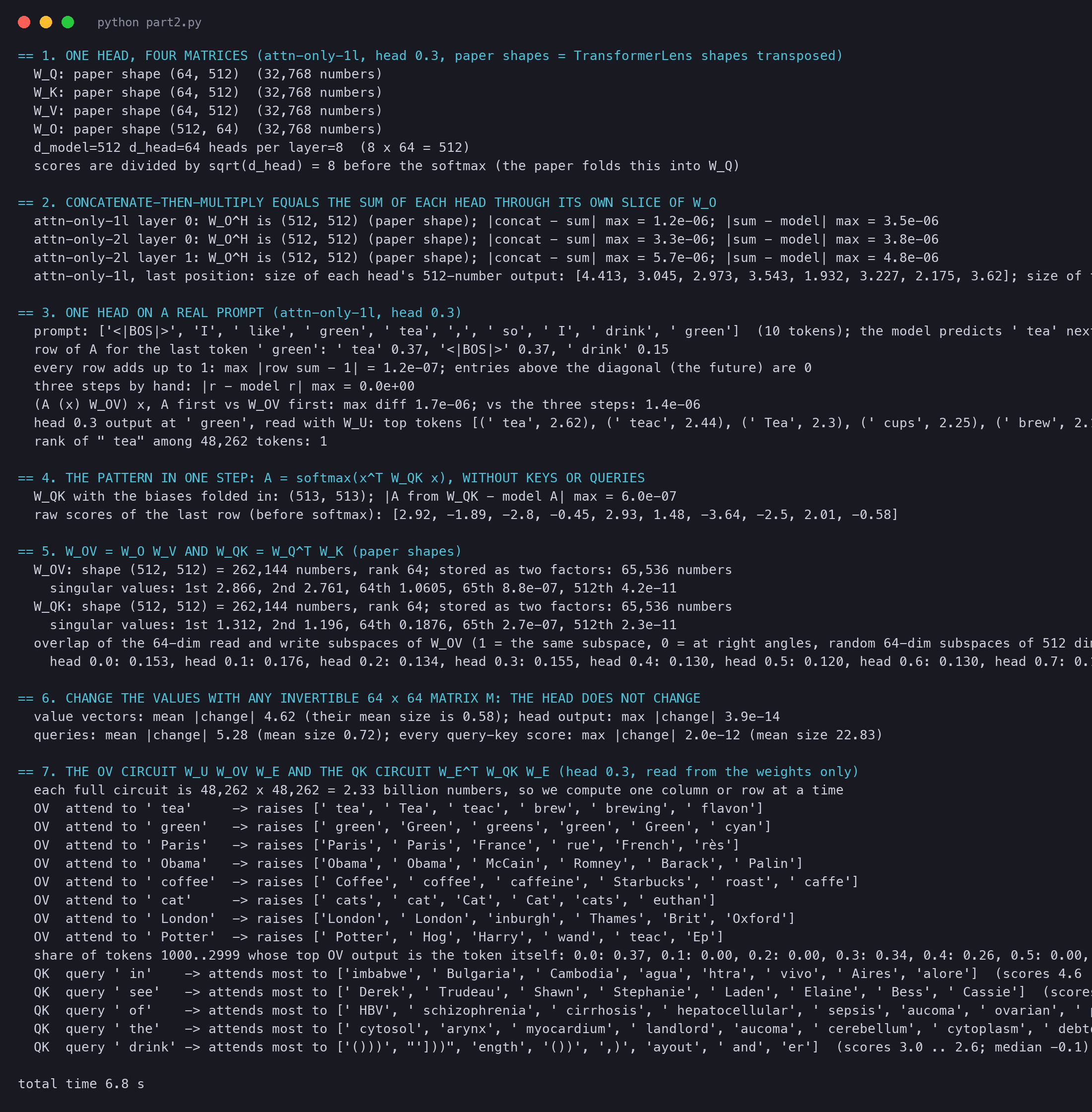
One detail differs between the paper and the code. Real implementations, including TransformerLens, divide every score by $\sqrt{d_\text{head}}=8$ before the softmax. The paper leaves this out, because the division can be folded into $W_{\mathrm{Q}}$. Here are the four matrices of head 0.3 in the paper's shapes, as printed by our script:

== 1. ONE HEAD, FOUR MATRICES (attn-only-1l, head 0.3, paper shapes = TransformerLens shapes transposed)
  W_Q: paper shape (64, 512)  (32,768 numbers)
  W_K: paper shape (64, 512)  (32,768 numbers)
  W_V: paper shape (64, 512)  (32,768 numbers)
  W_O: paper shape (512, 64)  (32,768 numbers)
  d_model=512 d_head=64 heads per layer=8  (8 x 64 = 512)
  scores are divided by sqrt(d_head) = 8 before the softmax (the paper folds this into W_Q)

Heads are independent and additive#

In Part 1 we wrote a layer as "every head adds its output to the stream". But that is not how the original transformer paper describes a layer. The paper first shows that the two descriptions are the same.

The derivation#

Take a layer with eight heads. Each head $h$ has a result vector $r^h$ of 64 numbers. The usual description stacks the eight result vectors into one long vector of $8\times64=512$ numbers. It then multiplies this long vector by one output matrix $W_{\mathrm{O}}^H$, which is 512 × 512.

To see why this equals a sum, we need one fact about any matrix-vector product. Multiplying a matrix $W$ by a vector $v$ is the same as adding up the columns of $W$, each one scaled by the matching number in $v$:

Here $W_{:,k}$ means column $k$ of $W$. You can check this on any small example: row $i$ of the answer is $\sum_k W_{ik}v_k$, which is exactly row $i$ of the sum of scaled columns.

Now apply this to $W_{\mathrm{O}}^H$ and the stacked vector. The first 64 numbers of the stacked vector belong to head 1, and they only ever multiply the first 64 columns of $W_{\mathrm{O}}^H$. The next 64 numbers belong to head 2, and they only multiply the next 64 columns, and so on. So we can group the sum of columns by head. The first 64 columns of $W_{\mathrm{O}}^H$ form a 512 × 64 block, which we call $W_{\mathrm{O}}^{1}$. The next 64 columns form $W_{\mathrm{O}}^{2}$, and so on. With two heads, the product reads:

With eight heads the sum simply has eight terms. In words, the big output matrix is just the eight small output matrices placed side by side. Multiplying by it is the same as letting every head write on its own and adding the results.

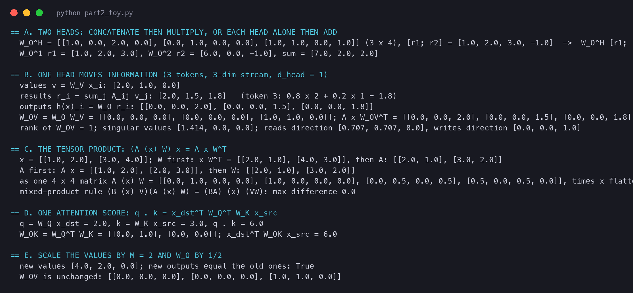
A toy example. Our toy script uses a 3-number stream and two heads with 2-number results. Head 1 has $r^1=(1,2)$ and head 2 has $r^2=(3,-1)$. The figure works it out both ways.

On the real model. Our script takes the eight result vectors that TransformerLens stores (hook_z), stacks them, and multiplies by the big matrix. It also multiplies each head by its own slice of $W_{\mathrm{O}}$ and adds the eight answers. Finally it compares both with what the model really added to the stream:

z = cache['blocks.0.attn.hook_z'][0]                 # [10 positions, 8 heads, 64]: every r^h
big = z.reshape(10, 512) @ model.W_O[0].reshape(512, 512)          # stack, then one multiply
summed = sum(z[:, h] @ model.W_O[0, h] for h in range(8))          # each head alone, then add

== 2. CONCATENATE-THEN-MULTIPLY EQUALS THE SUM OF EACH HEAD THROUGH ITS OWN SLICE OF W_O
  attn-only-1l layer 0: W_O^H is (512, 512) (paper shape); |concat - sum| max = 1.2e-06; |sum - model| max = 3.5e-06
  attn-only-2l layer 0: W_O^H is (512, 512) (paper shape); |concat - sum| max = 3.3e-06; |sum - model| max = 3.8e-06
  attn-only-2l layer 1: W_O^H is (512, 512) (paper shape); |concat - sum| max = 5.7e-06; |sum - model| max = 4.8e-06

In all three layers the largest difference is a few millionths, which is rounding noise. So the paper's picture is exact: a layer is eight heads that each write on their own.

Why this is useful. A head in a layer never sees what the other heads in the same layer write. They all read the same stream, and their outputs are only added afterwards. So we can study one head at a time, which is what the rest of this part does. This is also why, in Part 1, the final stream split cleanly into one piece per head.

A head moves information#

If heads work alone, what does each one do? The paper's answer is short.

Remember from Part 1 that every position has its own residual stream. Before attention, the stream at position 9 only knows about token 9. A head is the only part of this model that can carry information across positions. The paper draws it like this:

The three steps#

The paper then writes a head as three steps. These are the same equations as in our first section, but now each step is labelled by what it does.

Let us run the three steps by hand on a tiny head. The stream has 3 numbers per token, and there are 3 tokens. The head has $d_\text{head}=1$, so every value is a single number. Its matrices are $W_{\mathrm{V}}=(1,1,0)$, which adds up dimensions 1 and 2, and $W_{\mathrm{O}}=(0,0,1)^\top$, which writes into dimension 3. The attention pattern is given.

Look at token 3. Its own stream is $(0,0,1)$, and its own value is 0. Yet after the head, dimension 3 of its stream has received 1.8. That number came almost entirely from token 1, which had a 2 in its first dimension. The information "token 1 has something in dimension 1" has moved to token 3, and it has landed in dimension 3. This is the paper's picture in three small tables.

A real attention pattern#

Now the real head. We run attn-only-1l on our prompt and keep the pattern of head 0.3:

logits, cache = model.run_with_cache('I like green tea, so I drink green')
A = cache['blocks.0.attn.hook_pattern'][0, 3]       # [10, 10]: head 0.3, row = destination, column = source

== 3. ONE HEAD ON A REAL PROMPT (attn-only-1l, head 0.3)
  prompt: ['<|BOS|>', 'I', ' like', ' green', ' tea', ',', ' so', ' I', ' drink', ' green']  (10 tokens); the model predicts ' tea' next
  row of A for the last token ' green': ' tea' 0.37, '<|BOS|>' 0.37, ' drink' 0.15
  every row adds up to 1: max |row sum - 1| = 1.2e-07; entries above the diagonal (the future) are 0

The first token, <|BOS|>, is a special "beginning of text" token that TransformerLens adds in front of every prompt. Many rows put a lot of weight on it. A head must spend its weights somewhere, because each row adds up to 1, and the first token is a common place to park weight that has nothing better to do.

The interesting row is the last one. Standing on the second " green", head 0.3 reads " tea" with weight 0.37. That is the token the model predicts next. So the head looks back at the word that followed "green" last time. What does it carry over? We can check by reading the head's output at the last position through the unembedding $W_{\mathrm{U}}$, as in Part 1:

  head 0.3 output at ' green', read with W_U: top tokens [(' tea', 2.62), (' teac', 2.44), (' Tea', 2.3), (' cups', 2.25), (' brew', 2.16)]
  rank of " tea" among 48,262 tokens: 1

Out of 48,262 tokens, the one this head pushes up most is " tea". The head moved "tea" from position 4 to position 9. In the paper's words, it moved information from one residual stream to another.

The two sides of x, and the tensor product#

The paper now asks a natural question. Each of the three steps is a matrix multiplication, so why not collapse them into one step? The answer needs one new piece of notation, the tensor product. This section explains it without any jargon.

x is a table, and it has two sides#

So far $x_i$ was one token's vector. Now put all the tokens together. Stack the vectors as the rows of one table $x$. For our prompt, $x$ has 10 rows (one per token) and 512 columns (one per dimension of the stream).

A matrix can multiply this table from two sides.

• Multiplying from the left, as in $A\,x$, mixes the rows. Row $i$ of $A\,x$ is $\sum_j A_{ij}\,x_j$, a weighted mix of the tokens. This is what the attention pattern does.
• Multiplying from the right, as in $x\,W^\top$, changes each row on its own. Row $i$ of $x\,W^\top$ is $W x_i$. This is what $W_{\mathrm{V}}$ and $W_{\mathrm{O}}$ do.

One formula for the whole head#

Now collapse the three steps. Start from step 3 and substitute steps 2 and 1 into it:

The number $A_{ij}$ is just a scalar, so it can move past the matrices. And $W_{\mathrm{O}}$ can move inside the sum, because matrix multiplication spreads over a sum. This gives:

Read this slowly. For each source token $j$, the matrix $W_{\mathrm{O}} W_{\mathrm{V}}$ turns $x_j$ into "what token $j$ sends". Then $A_{ij}$ decides how much of it token $i$ receives. The two parts never mix: $A$ only has position indices, and $W_{\mathrm{O}} W_{\mathrm{V}}$ only acts inside a vector.

In table form, using the two sides from above, the whole head is:

The paper gives the product $W_{\mathrm{O}} W_{\mathrm{V}}$ its own name, $W_{\mathrm{OV}}$. It is 512 × 512.

The tensor product, made plain#

The paper writes the same thing with a new symbol, $\otimes$. For any position-mixing matrix $A$ and any per-token matrix $W$, it defines

That is all the symbol means here: "mix the rows with $A$, and change each row with $W$". With this notation, the whole head is

The appendix of the paper lists the practical rules:

Why does the order not matter? Matrix multiplication is associative: $(A\,x)\,W^\top$ and $A\,(x\,W^\top)$ are the same table. So you can mix first and transform second, or the other way round. Here is a toy with two tokens and two dimensions. $A$ lets token 2 take half of each token, and $W$ swaps the two numbers of a token.

You can also flatten the table into one long vector of 4 numbers. Then $A\otimes W$ becomes one ordinary 4 × 4 matrix, the Kronecker product. Our toy script builds it and gets the same answer:

  as one 4 x 4 matrix A (x) W = [[0.0, 1.0, 0.0, 0.0], [1.0, 0.0, 0.0, 0.0], [0.0, 0.5, 0.0, 0.5], [0.5, 0.0, 0.5, 0.0]], times x flattened [1.0, 2.0, 3.0, 4.0] = [2.0, 1.0, 3.0, 2.0]

The flat view is correct, but it hides the structure, so the paper (and this series) uses the two-sided view.

The paper's derivation, step by step#

The paper skips the algebra, so let us fill it in. The three steps, read from right to left, are:

Here $\text{Id}$ is the identity matrix, which changes nothing. So $\text{Id}\otimes W_{\mathrm{V}}$ means "do not mix tokens; multiply each token by $W_{\mathrm{V}}$". The mixed-product property says how two tensor products combine:

It follows from our definition in two lines. Apply $C\otimes D$ first, then $A\otimes B$:

The last step uses $D^\top B^\top=(BD)^\top$, a standard rule for transposes. The right side is exactly $\big((AC)\otimes(BD)\big)\,x$. Now combine the first two factors of the head:

Then combine the result with the last factor:

That is the paper's result. The identities "collapse" because multiplying by $\text{Id}$ changes nothing.

On the real model. We computed head 0.3's output on our prompt in three ways: the three steps, the formula with $A$ applied first, and the formula with $W_{\mathrm{OV}}$ applied first.

W_OV_row = model.W_V[0, 3] @ model.W_O[0, 3]     # TransformerLens stores the transpose: this is W_OV^T
first_A = (A @ X) @ W_OV_row                      # mix tokens first, then change each token
first_W = A @ (X @ W_OV_row)                      # change each token first, then mix

  three steps by hand: |r - model r| max = 0.0e+00
  (A (x) W_OV) x, A first vs W_OV first: max diff 1.7e-06; vs the three steps: 1.4e-06

All three agree up to rounding noise. Here X is the stream as the head sees it, after the leftover part of layer norm from Part 1.

The pattern in one step: the QK matrix#

We have collapsed the "what" part. The paper does the same for the "where" part, the attention pattern.

The derivation#

Write the score of one pair as a product of matrices. A dot product $a\cdot b$ is the same as $a^\top b$, so:

The last step uses the transpose rule again: $(W_{\mathrm{Q}} x_i)^\top=x_i^\top {W_{\mathrm{Q}}}^{\top}$. The paper names the middle product:

Its shape is $(512\times64)(64\times512)=512\times512$. With it, every score is $s_{ij}=x_i^\top W_{\mathrm{QK}}\,x_j$. The paper writes the whole table of scores at once as $x^\top W_{\mathrm{QK}}\,x$ (with the tokens as the columns of $x$), and then applies the masked softmax.

A toy example. Let the stream have 2 numbers and the head 1 number. The query reads dimension 1, $W_{\mathrm{Q}}=(1,0)$, and the key reads dimension 2, $W_{\mathrm{K}}=(0,1)$. The destination token is $(2,0)$ and the source token is $(0,3)$.

The single entry 1 in $W_{\mathrm{QK}}$ sits in row 1, column 2. It means "dimension 1 of the destination meets dimension 2 of the source". Every entry of a real $W_{\mathrm{QK}}$ has this meaning: how much one direction at the destination wants to meet another direction at the source.

On the real model. The real head also has biases on its queries and keys. Part 1 showed that a bias is just one more column for an always-1 input. So we add a 513th dimension that is always 1, put the biases there, and compute the whole pattern from a single 513 × 513 matrix:

Xt  = torch.cat([X, ones], 1)                                  # [10, 513]: an always-1 column for the biases
WQt = torch.cat([W_Q, b_Q[None]], 0); WKt = torch.cat([W_K, b_K[None]], 0)
scores = Xt @ (WQt @ WKt.T) @ Xt.T / 8                         # every query-key score in one product

== 4. THE PATTERN IN ONE STEP: A = softmax(x^T W_QK x), WITHOUT KEYS OR QUERIES
  W_QK with the biases folded in: (513, 513); |A from W_QK - model A| max = 6.0e-07
  raw scores of the last row (before softmax): [2.92, -1.89, -2.8, -0.45, 2.93, 1.48, -3.64, -2.5, 2.01, -0.58]

The pattern from one matrix matches the model's pattern to within 0.0000006. Look at the raw scores of the last row. " tea" (position 4) scores 2.93 and BOS scores 2.92. Nearly equal scores give nearly equal weights, which is why both got 0.37.

Why "horribly inefficient"? $W_{\mathrm{QK}}$ has $512\times512=262{,}144$ numbers, while $W_{\mathrm{Q}}$ and $W_{\mathrm{K}}$ together have $65{,}536$. Multiplying a token by the big matrix costs about four times as much as going through the two thin ones. So code keeps the factors. But for reading a head, the product is the natural object.

What the new form shows#

The paper then lists what this way of writing a head reveals. We take its observations one at a time.

Heads move information, so the stream holds copied information#

The first observation repeats the main idea: heads move information from one token's stream to another's. The paper draws a consequence. The residual stream is often called a "contextual word embedding", as if it only described the current token. But after a head has run, the stream at a token also contains information copied from other tokens, in its own subspace. We saw exactly this: after head 0.3, the stream at the last " green" contains a direction that means "tea".

Two linear operations, and only one is non-linear#

Why is the head non-linear at all? Because the pattern is computed from the input. If you double $x$, the scores grow four times (both $x_i$ and $x_j$ double), and the softmax of the new scores is a different pattern. But once $A$ is fixed, $h(x)=A\,x\,{W_{\mathrm{OV}}}^{\top}$ is linear in $x$: doubling $x$ doubles the output.

W_OV and W_QK are low-rank#

The paper's footnote on this observation explains how $W_{\mathrm{OV}}$ chooses what to read and where to write. It uses the singular value decomposition $W_{\mathrm{OV}}=USV$. "Since $d_\text{head}<d_\text{model}$, $W_{\mathrm{OV}}$ is low-rank and only a subset of the diagonal entries in $S$ are non-zero." The right singular vectors "describe which subspace of the residual stream being attended to is read in", and the left singular vectors "describe what subspace of the destination residual stream they are written to".

First, why can the rank of $W_{\mathrm{OV}}$ be at most 64? Apply it to any vector $x$:

The bracket $W_{\mathrm{V}} x$ has only 64 numbers. So the output is $W_{\mathrm{O}}$ times some 64-number vector. That is always a mix of the 64 columns of $W_{\mathrm{O}}$. Every possible output lies in a space of at most 64 dimensions, out of 512. The same argument works for $W_{\mathrm{QK}}={W_{\mathrm{Q}}}^{\top} W_{\mathrm{K}}$.

A toy example. In our three-step toy, $W_{\mathrm{OV}}=W_{\mathrm{O}} W_{\mathrm{V}}$ is a 3 × 3 matrix whose last row is $(1,1,0)$ and whose other rows are zero. Its rank is 1. The SVD from the toy script finds one singular value, 1.414. Its input direction is $(0.707,0.707,0)$, which is "dimensions 1 and 2 together". Its output direction is $(0,0,1)$, which is "dimension 3". In words: this head reads dimensions 1 and 2, and writes into dimension 3. Those are two different subspaces, just like the paper's drawing.

On the real model. Our script computes the SVD of both matrices of head 0.3:

== 5. W_OV = W_O W_V AND W_QK = W_Q^T W_K (paper shapes)
  W_OV: shape (512, 512) = 262,144 numbers, rank 64; stored as two factors: 65,536 numbers
    singular values: 1st 2.866, 2nd 2.761, 64th 1.0605, 65th 8.8e-07, 512th 4.2e-11
  W_QK: shape (512, 512) = 262,144 numbers, rank 64; stored as two factors: 65,536 numbers
    singular values: 1st 1.312, 2nd 1.196, 64th 0.1876, 65th 2.7e-07, 512th 2.3e-11

There is a sharp cliff after value 64. The 65th singular value is about a million times smaller than the 64th, which means it is zero up to rounding. So each 512 × 512 matrix really lives in 64 dimensions.

Does the head read and write in different places, as the paper's drawing says? We measured the overlap between the 64-dimensional read subspace and the 64-dimensional write subspace of each head's $W_{\mathrm{OV}}$. The score is 1 if they are the same subspace and 0 if they are at right angles. Two random 64-dimensional subspaces of a 512-dimensional space score about $64/512=0.125$.

  overlap of the 64-dim read and write subspaces of W_OV (1 = the same subspace, 0 = at right angles, random 64-dim subspaces of 512 dims: 0.125)
    head 0.0: 0.153, head 0.1: 0.176, head 0.2: 0.134, head 0.3: 0.155, head 0.4: 0.130, head 0.5: 0.120, head 0.6: 0.130, head 0.7: 0.155

Every head scores between 0.120 and 0.176, close to the random 0.125. So the heads read from one part of the stream and write to a mostly different part. For head 0.3 this makes sense. It reads "which token is this" (an embedding direction) and writes "which token should come next" (an unembedding direction). Part 1 showed that these are different, because $W_{\mathrm{U}}$ is not the inverse of $W_{\mathrm{E}}$.

Queries, keys and values are superficial#

What does "reparametrize" mean? Take any invertible 64 × 64 matrix $M$. Replace $W_{\mathrm{V}}$ by $M\,W_{\mathrm{V}}$ and $W_{\mathrm{O}}$ by $W_{\mathrm{O}} M^{-1}$. The value vectors are now completely different. But their product is unchanged:

The same trick works for queries and keys, with $M$ on one side and the transpose of $M^{-1}$ on the other. In our toy, scaling every value by $M=2$ and $W_{\mathrm{O}}$ by one half gives new values $(4,2,0)$ but exactly the same outputs.

On the real head we used a random 64 × 64 matrix. The value vectors and queries change completely, and the head does not change at all:

== 6. CHANGE THE VALUES WITH ANY INVERTIBLE 64 x 64 MATRIX M: THE HEAD DOES NOT CHANGE
  value vectors: mean |change| 4.62 (their mean size is 0.58); head output: max |change| 3.9e-14
  queries: mean |change| 5.28 (mean size 0.72); every query-key score: max |change| 2.0e-12 (mean size 22.83)

The values moved by 4.62 on average, eight times their usual size. The head's output moved by less than $10^{-13}$. So "dimension 17 of the value vector" means nothing on its own, just as "dimension 7 of the stream" meant nothing in Part 1. The meaningful objects are $W_{\mathrm{OV}}$ and $W_{\mathrm{QK}}$.

Products of heads behave like heads#

The last observation looks ahead. By the mixed-product property, two heads applied one after the other combine like this:

The result has the same shape as one head: a pattern $A^2A^1$ and an OV matrix $W_{\mathrm{OV}}^2W_{\mathrm{OV}}^1$. The paper calls it a virtual attention head. It only appears when there are two layers, so Part 5 comes back to it. Our toy script checked the property itself on 2 × 2 matrices, with a difference of exactly 0.

From weights to tokens: the QK and OV circuits#

So far $W_{\mathrm{QK}}$ and $W_{\mathrm{OV}}$ act on the 512-number stream. A stream vector is hard to read. A token is easy to read. The paper's last step for a single head is to attach the embedding and the unembedding, so that both matrices go from tokens to tokens.

The derivation#

Take a one-layer model and ignore the position embedding for now, as the paper does. Then the stream that the head reads at position $j$ is just the token's embedding, $x_j=W_{\mathrm{E}}\,t_j$, where $t_j$ is the one-hot vector of the token (Part 1).

The QK circuit. Put $x_i=W_{\mathrm{E}} t_i$ and $x_j=W_{\mathrm{E}} t_j$ into the score:

The matrix in the bracket is the QK circuit. It multiplies a 48,262 × 512 matrix, a 512 × 512 matrix and a 512 × 48,262 matrix, so its shape is 48,262 × 48,262. Multiplying by two one-hot vectors just picks one entry. So the entry in row $a$, column $b$ is the score that a destination token $a$ gives to a source token $b$. It is a table of "how much does token $a$ want to read token $b$".

The OV circuit. The head adds $h(x)_i$ to the stream, and in a one-layer model the stream goes straight to the unembedding. So the head's effect on the logits at position $i$ is $W_{\mathrm{U}}\,h(x)_i$. Using our one-line formula for the head:

The matrix in the bracket is the OV circuit, also $48{,}262\times48{,}262$. Column $b$ of it is a list of 48,262 logit changes. It answers: "if this head reads token $b$ with full weight, which next tokens does it push up?"

Look at the formula for $W_{\mathrm{U}} h(x)_i$ once more. It is the sum over source tokens of (weight from QK) × (effect from OV). The QK circuit only affects the weights $A_{ij}$. The OV circuit only affects what each source contributes. That is the "completely separable" of the paper, now written in tokens.

Why splitting is useful. Each circuit is a fixed table that can be read from the weights alone, without any input text. The QK circuit is bilinear (a score between two tokens), and the OV circuit is linear (an effect of one token). Both are easy kinds of function. The only hard part, the softmax, sits between them and does not change what either table says.

Reading the OV circuit of head 0.3#

A full circuit has $48{,}262^2\approx2.33$ billion entries, which is too many to store comfortably. So we compute one column at a time. There is one practical step. The leftover layer norm (Part 1) divides each token's vector by its size before the head reads it. So we scale every embedding to that same size first. A scale does not change which outputs come top in a column, but it keeps different tokens comparable.

WE = model.W_E - model.W_E.mean(1, keepdim=True)
WE = WE / WE.std(1, keepdim=True)                                 # what layer norm does to each token
t = model.to_single_token(' tea')
col = (WE[t] @ model.W_V[0, 3] @ model.W_O[0, 3]) @ model.W_U     # column ' tea' of W_U W_OV W_E
print(model.to_str_tokens(col.topk(6).indices))

== 7. THE OV CIRCUIT W_U W_OV W_E AND THE QK CIRCUIT W_E^T W_QK W_E (head 0.3, read from the weights only)
  each full circuit is 48,262 x 48,262 = 2.33 billion numbers, so we compute one column or row at a time
  OV  attend to ' tea'     -> raises [' tea', ' Tea', ' teac', ' brew', ' brewing', ' flavon']
  OV  attend to ' green'   -> raises [' green', 'Green', ' greens', 'green', ' Green', ' cyan']
  OV  attend to ' Paris'   -> raises ['Paris', ' Paris', 'France', ' rue', 'French', 'rès']
  OV  attend to ' Obama'   -> raises ['Obama', ' Obama', ' McCain', ' Romney', ' Barack', ' Palin']
  OV  attend to ' coffee'  -> raises [' Coffee', ' coffee', ' caffeine', ' Starbucks', ' roast', ' caffe']
  OV  attend to ' cat'     -> raises [' cats', ' cat', 'Cat', ' Cat', 'cats', ' euthan']
  OV  attend to ' London'  -> raises ['London', ' London', 'inburgh', ' Thames', 'Brit', 'Oxford']
  OV  attend to ' Potter'  -> raises [' Potter', ' Hog', 'Harry', ' wand', ' teac', 'Ep']

The pattern is clear. Whatever token head 0.3 reads, it pushes up that same token and close relatives: other spellings, plurals, related words ("Paris" brings "France", "Obama" brings "McCain"). This is a copying head. We can count it over 2,000 ordinary tokens (numbers 1,000 to 2,999):

  share of tokens 1000..2999 whose top OV output is the token itself: 0.0: 0.37, 0.1: 0.00, 0.2: 0.00, 0.3: 0.34, 0.4: 0.26, 0.5: 0.00, 0.6: 0.12, 0.7: 0.00

For head 0.3, the top output is the token itself for 34% of tokens. Heads 0.0 and 0.4 copy too; heads 0.1, 0.2, 0.5 and 0.7 almost never do. So the eight heads of one layer really do different jobs, and the OV circuit tells them apart from the weights alone.

This explains our prompt. On the last " green", the QK side made the head read " tea", and the OV side turned "I read tea" into "push up tea". The output we read earlier (tea +2.62) is built the same way: this column of the OV circuit, weighted by 0.37, plus the columns of the other tokens the head read, each weighted by its own attention. In the real model the values also carry a position part, so the match is not exact, but the mechanism is the same.

Reading the QK circuit of head 0.3#

For the QK circuit we fix a destination token and compute its row: the score it gives to every one of the 48,262 possible source tokens. This leaves out positions and biases, so it shows only the token part of the score.

K = WE @ model.W_K[0, 3]                                  # the key of every token: [48262, 64]
q = WE[model.to_single_token(' in')] @ model.W_Q[0, 3]    # the query of ' in'
row = K @ q / 8                                           # row ' in' of W_E^T W_QK W_E

  QK  query ' in'    -> attends most to ['imbabwe', ' Bulgaria', ' Cambodia', 'agua', 'htra', ' vivo', ' Aires', 'alore']  (scores 4.6 .. 3.9; median 0.5)
  QK  query ' see'   -> attends most to [' Derek', ' Trudeau', ' Shawn', ' Stephanie', ' Laden', ' Elaine', ' Bess', ' Cassie']  (scores 2.8 .. 2.7; median 0.2)
  QK  query ' of'    -> attends most to [' HBV', ' schizophrenia', ' cirrhosis', ' hepatocellular', ' sepsis', 'aucoma', ' ovarian', ' psori']  (scores 2.7 .. 2.4; median 0.4)
  QK  query ' the'   -> attends most to [' cytosol', 'arynx', ' myocardium', ' landlord', 'aucoma', ' cerebellum', ' cytoplasm', ' debtor']  (scores 2.8 .. 2.5; median 0.5)
  QK  query ' drink' -> attends most to ['()))', "']))", 'ength', '())', ',)', 'ayout', ' and', 'er']  (scores 3.0 .. 2.6; median -0.1)

Most rows make sense once you pair them with the OV circuit. Standing on " in", the head looks for an earlier place name, and its OV circuit then copies that place: "... Bulgaria ... in" → "Bulgaria". Standing on " see", it looks for an earlier first name and copies it. The top scores (2.7 to 4.6) sit far above the typical score of each row, which is between 0.2 and 0.5, so these choices are strong.

Not every row is this clean. The row for " drink" is topped by pieces of code punctuation. This is honest data: a single head has 64 dimensions to serve 48,262 tokens, and the token-only view leaves out positions and biases. Part 4 shows how the paper summarises whole circuits rather than picking rows, and where the simple reading breaks down.

Next, in Part 3: we put the pieces together. The paper's path expansion trick multiplies out the whole model, embedding, heads and unembedding, and turns it into a sum of end-to-end paths: the direct path from Part 1, plus one term per head built from exactly the QK and OV circuits of this part. Part 4 then reads those terms for the one-layer model as skip-trigrams, with the paper's results on copying and its "bugs".

Run it yourself

The two scripts behind this part are circuits_part2.py (every real-model number: the shapes, the head-sum check on both models, the attention pattern, the tensor form, the one-step pattern, the ranks and singular values, the reparametrisation test, and the OV and QK circuits) and circuits_part2_toy.py (the hand-sized examples). The first one downloads attn-only-1l and attn-only-2l from Hugging Face the first time, then runs on the CPU in under 10 seconds.

TransformerLens 4 replaced the HookedTransformer class used here, so install a 3.x version:

bashCopy

pip install torch "transformer_lens<4"
python circuits_part2.py        # writes results/part2.json and results/part2_stdout.txt
python circuits_part2_toy.py    # writes results/part2_toy.json

References#

The paper

1. N. Elhage, N. Nanda, C. Olsson, T. Henighan, N. Joseph, B. Mann, A. Askell, Y. Bai, A. Chen, T. Conerly, N. DasSarma, D. Drain, D. Ganguli, Z. Hatfield-Dodds, D. Hernandez, A. Jones, J. Kernion, L. Lovitt, K. Ndousse, D. Amodei, T. Brown, J. Clark, J. Kaplan, S. McCandlish, C. Olah. A Mathematical Framework for Transformer Circuits. Transformer Circuits Thread, Anthropic, 22 December 2021. The screenshots in this part come from this page.
2. Transformer Circuits Thread, the series of articles this paper opened.

Related papers

3. A. Vaswani, N. Shazeer, N. Parmar, J. Uszkoreit, L. Jones, A. N. Gomez, Ł. Kaiser, I. Polosukhin. Attention Is All You Need. NeurIPS 2017. The original description of multi-head attention, with the stacked output matrix.
4. C. Olsson, N. Elhage, N. Nanda, et al. In-context Learning and Induction Heads. 2022 (web version). The follow-up that reads QK and OV circuits in larger models.
5. C. Olah, N. Cammarata, L. Schubert, G. Goh, M. Petrov, S. Carter. Zoom In: An Introduction to Circuits. Distill, 2020. The earlier work on image models that gave "circuits" its meaning.

Tools and models

6. N. Nanda, J. Bloom, and contributors. TransformerLens, the library used for every experiment; version 3.9.0.
7. Model cards: NeelNanda/Attn_Only_1L512W_C4_Code (attn-only-1l) and NeelNanda/Attn_Only_2L512W_C4_Code (attn-only-2l).
8. Code for this part: circuits_part2.py and circuits_part2_toy.py.