SAM, explained · Part 4 of 6 · Covers §4, §5, §6, Figures 2, 5, 6, 7, Tables 1, 2, 6, Appendix B, Appendix C
The Data Engine and SA-1B
How SAM first helped people draw masks, and then drew 1.1 billion masks by itself. We rebuild its automatic step on two photos and check each filter.
Segment Anything. Alexander Kirillov, Eric Mintun, Nikhila Ravi, Hanzi Mao, Chloe Rolland, Laura Gustafson, Tete Xiao, Spencer Whitehead, Alexander C. Berg, Wan-Yen Lo, Piotr Dollár, Ross Girshick. ICCV 2023, 2023. arXiv:2304.02643
SAM learned from 1.1 billion masks, and SAM drew almost all of them itself. This part shows how a model can make its own training data, how the team checked that data, and what the data contains. We also rebuild the machine that drew the masks, with the released model, on two photos.
Part 1 gave the three stages in short. The picture below collects every number that Section 4 gives for them.
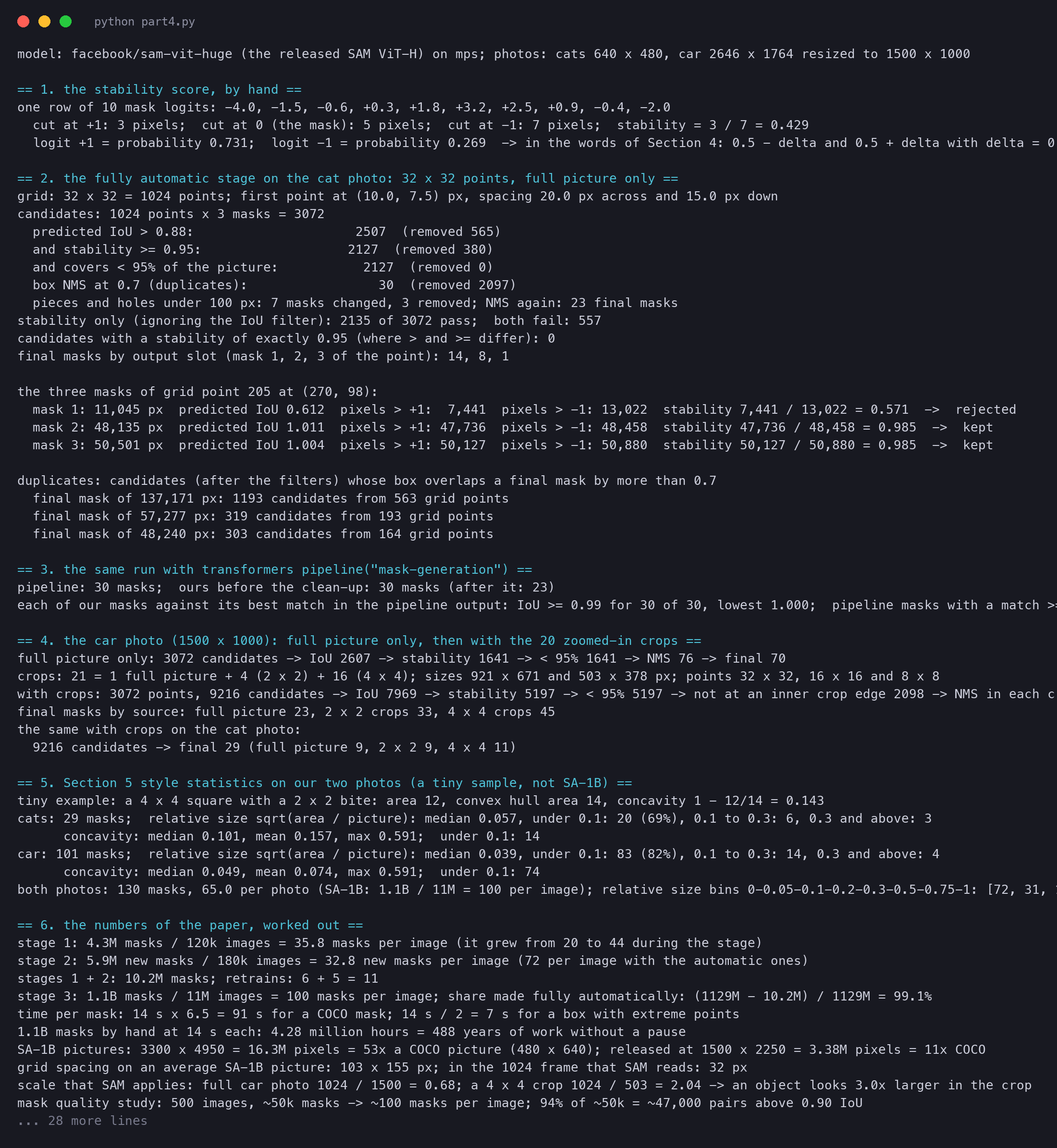
The three stages of the data engine with the numbers of Section 4. People drew the masks of stages 1 and 2 with SAM's help: 10.2 million masks. SAM alone drew the 1.1 billion masks of stage 3.
stage 1: 4.3M masks / 120k images = 35.8 masks per image (it grew from 20 to 44 during the stage)time per mask: 14 s x 6.5 = 91 s for a COCO mask; 14 s / 2 = 7 s for a box with extreme points1.1B masks by hand at 14 s each: 4.28 million hours = 488 years of work without a pause
The paper gives only the ratios; the 91 and 7 seconds are our arithmetic from them. The last line shows why the engine could not stay manual. Even at the best speed of stage 1, one person would need 488 years to draw SA-1B.
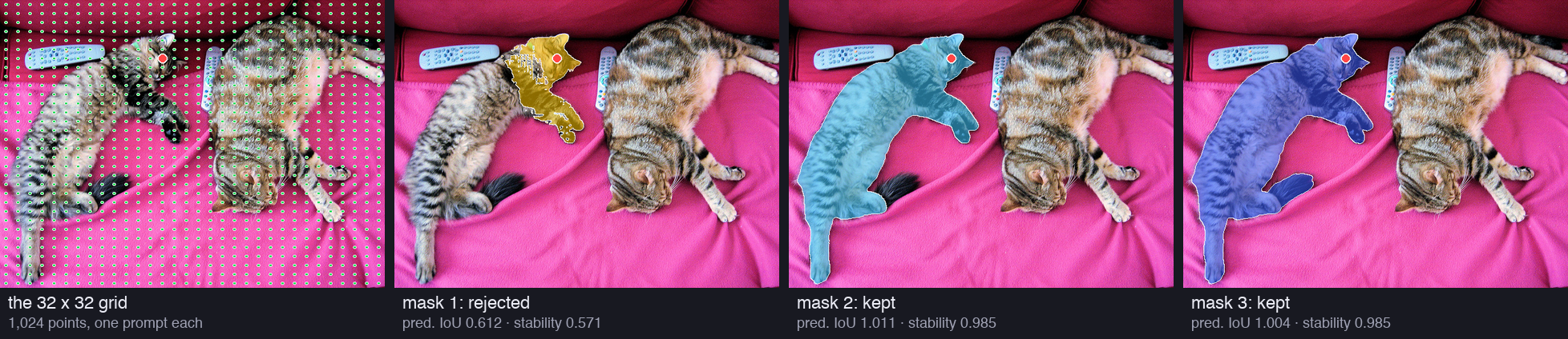
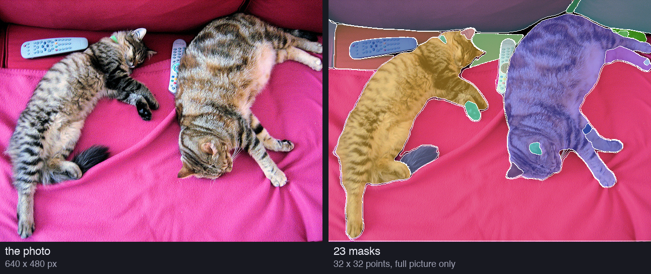
We did the same on the cat photo of the earlier parts, with the released ViT-H. Each grid point is one prompt, and each prompt gives three masks:
The 32 × 32 grid on the cat photo, and the three masks of one grid point (red dot). Each mask carries two numbers, the predicted IoU and the stability; the filters below use them.
plain text
grid: 32 x 32 = 1024 points; first point at (10.0, 7.5) px, spacing 20.0 px across and 15.0 px downcandidates: 1024 points x 3 masks = 3072
So one photo gives 3,072 candidate masks. Most are poor or are copies of each other. The next lines of the paper say how SAM keeps the good ones.
Appendix B gives the exact rules. We take them one at a time and apply each to our candidates.
The IoU head of Part 3 predicts how well each mask fits the object it covers. A score of 0.95 means "I think this mask overlaps the true object with an IoU of about 0.95". Filter 1 keeps only masks with a predicted IoU above 0.88. On the cat photo:
plain text
predicted IoU > 0.88: 2507 (removed 565)
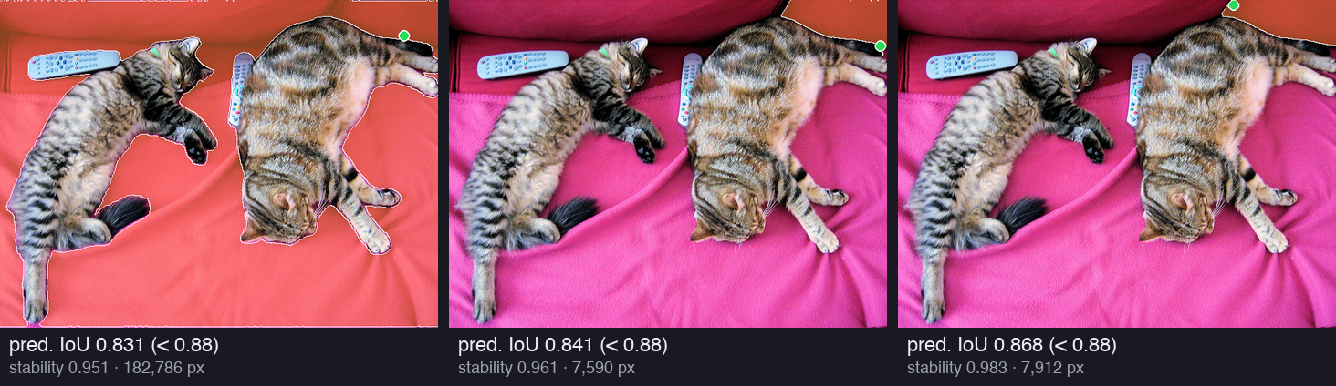
565 candidates fail. Here are three of them, from the lowest score upward:
Masks that filter 1 removes. Each has a predicted IoU under 0.88, though each is stable (stability 0.951 to 0.983). The green dot is the grid point that made the mask.
These masks are not nonsense, but they are not clear objects either. The first one is "everything except the cats". The other two are slices of the sofa at the edge of the photo. SAM gives them a low score, so they go.
The second filter asks a different question. Think of a drawing made with a soft pencil. If you trace it with a thin pen, then with a thick marker, a clear drawing gives almost the same shape twice. A fuzzy drawing gives two very different shapes. The stability score measures this.
SAM's mask is really a map of logits, one number for each pixel (Part 2 defined logits). The mask is the set of pixels with a logit above 0. Now cut the same map at +1 and at −1. The pixels above +1 form a smaller mask; the pixels above −1 form a larger mask. Every pixel above +1 is also above −1, so the small mask sits inside the large one.
ℓi is the logit of pixel i: positive means "inside", negative means "outside", and far from 0 means "sure".
Mc is the mask cut at the value c: all pixels with a logit above c.
∣M+1∣ counts the pixels that are clearly inside, and ∣M−1∣ counts the pixels that are inside or nearly inside.
Because M+1 is inside M−1, their intersection is M+1 and their union is M−1. So the IoU is a plain ratio of two counts.
S is near 1 when few pixels have a logit between −1 and +1. Those pixels are the unsure ones.
Section 4 describes the same rule with probabilities: cut "at 0.5 − δ and 0.5 + δ". A logit of +1 is a probability of 0.731, and a logit of −1 is 0.269. So the two descriptions agree with δ=0.231:
plain text
logit +1 = probability 0.731; logit -1 = probability 0.269 -> in the words of Section 4: 0.5 - delta and 0.5 + delta with delta = 0.231
A tiny example with one row of 10 pixels:
Ten pixels of one mask. Three pixels have a logit above +1 and seven have a logit above −1, so the stability is 3 / 7 = 0.429. The four pixels between the two cut-offs are the unsure edge.
plain text
one row of 10 mask logits: -4.0, -1.5, -0.6, +0.3, +1.8, +3.2, +2.5, +0.9, -0.4, -2.0
  cut at +1: 3 pixels;  cut at 0 (the mask): 5 pixels;  cut at -1: 7 pixels;  stability = 3 / 7 = 0.429
The mask itself has 5 pixels. But 4 of the 7 pixels near the mask sit between −1 and +1. A small change of the cut-off changes this mask a lot. The stability is 0.429, far under 0.95, and the mask is rejected. A real mask passes only if at most 5% of its "nearly inside" pixels are unsure.
Now the real thing. Here are the three masks of the grid point on the head of the left cat, the red dot in the grid picture.
Mask 1 covers the head and a front leg, with a ragged edge into the body. SAM is unsure where "the head" ends: 5,581 pixels lie between the two cut-offs. So S=7,441/13,022=0.571, and the mask fails. Its predicted IoU of 0.612 fails too. Masks 2 and 3 are the cat without its tail and the cat with its tail. Only 722 and 753 of their pixels are unsure, so both have S=0.985 and pass.
On the whole cat photo, filter 2 removes 380 of the 2,507 masks that passed filter 1:
plain text
and stability >= 0.95: 2127 (removed 380)
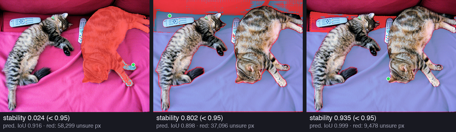
Here are three of them. Blue is the sure part (logit above +1); red is the unsure band (between −1 and +1):
Masks that filter 2 removes, although their predicted IoU is high (0.898 to 0.999). Blue: logit above +1. Red: logit between −1 and +1, the unsure pixels. The first mask is almost all doubt: 58,299 unsure pixels around a sure paw.
plain text
unstable example: stability 1,438 / 59,737 = 0.024, predicted IoU 0.916, 58,299 pixels between -1 and +1unstable example: stability 150,707 / 187,803 = 0.802, predicted IoU 0.898, 37,096 pixels between -1 and +1unstable example: stability 137,460 / 146,938 = 0.935, predicted IoU 0.999, 9,478 pixels between -1 and +1
The first example is a good lesson. The grid point sits on a paw of the right cat. SAM is sure about the paw, and it half believes that the whole cat belongs to the mask. The IoU head gives 0.916, so filter 1 lets it pass, and only the stability catches it.
The third example has a predicted IoU of 0.999, but its edge with the sofa is unsure. The two filters see different faults, which is why the paper uses both.
All 3,072 candidate masks of the cat photo, by predicted IoU and stability. The kept masks are in the top right box. Many masks have a high predicted IoU and a low stability, and the reverse: each filter removes masks that the other one keeps.
plain text
stability only (ignoring the IoU filter): 2135 of 3072 pass; both fail: 557
Sometimes a point on a plain background gives a mask of the whole picture. Such a mask says nothing, so masks that cover 95% or more of the picture go. On the cat photo, this filter removes nothing:
2,127 masks pass the three filters, but the photo shows only a few dozen objects. Many grid points sit on the same object, so they give the same mask again and again. The blanket under the cats is one region, but 563 grid points lie on it:
plain text
duplicates: candidates (after the filters) whose box overlaps a final mask by more than 0.7
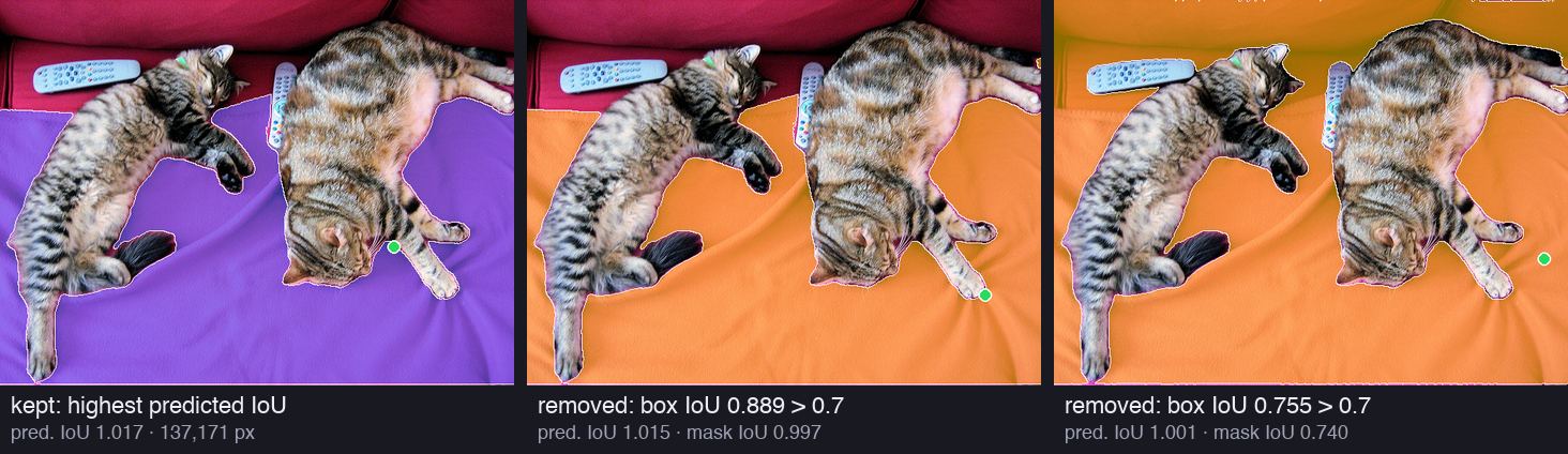
  final mask of 137,171 px: 1193 candidates from 563 grid points
  final mask of 57,277 px: 319 candidates from 193 grid points
  final mask of 48,240 px: 303 candidates from 164 grid points
Non-maximum suppression is a greedy rule from object detection. Sort all masks by score, from the best down. Take the best mask and keep it. Delete every other mask whose box overlaps it with an IoU above 0.7. Then take the best mask that is left, and repeat until no mask is left.
Think of a class photo where each student was photographed many times. You sort the photos by quality. You keep the best photo of the first face, and you throw away all other photos of that face. Then you go to the best photo that is left, which shows a new face.
Here is our version, in a few lines. It gives the same result as the NMS of torchvision; the script checks this on every crop.
python
def greedy_nms(boxes, scores, thr):
    order = scores.argsort(descending=True).tolist()      # best mask first
    keep, gone = [], set()
    iou = box_iou(boxes, boxes)                            # the IoU of every pair of boxes
    for i in order:
        if i in gone:
            continue
        keep.append(i)                                     # the best mask that is left
        for j in order:
            if j not in gone and j != i and iou[i, j] > thr:
                gone.add(j)                                # its copies go
    return keep
On the cat photo, NMS removes almost everything:
plain text
box NMS at 0.7 (duplicates): 30 (removed 2097)
NMS on the blanket. Left: the kept mask, with the highest predicted IoU among its copies. Middle and right: two of its 1,192 copies. Their boxes overlap the kept box by more than 0.7, so they go, even the right one, which also covers the sofa.
The right-hand example shows the price of the shortcut. Its mask covers the sofa too, so the masks overlap only by 0.740. But its box is almost the same as the box of the blanket, so NMS treats it as a copy. The scores of 1.015 and 1.017 are above 1; Part 3 explained that the IoU head can overshoot a little when it is very sure.
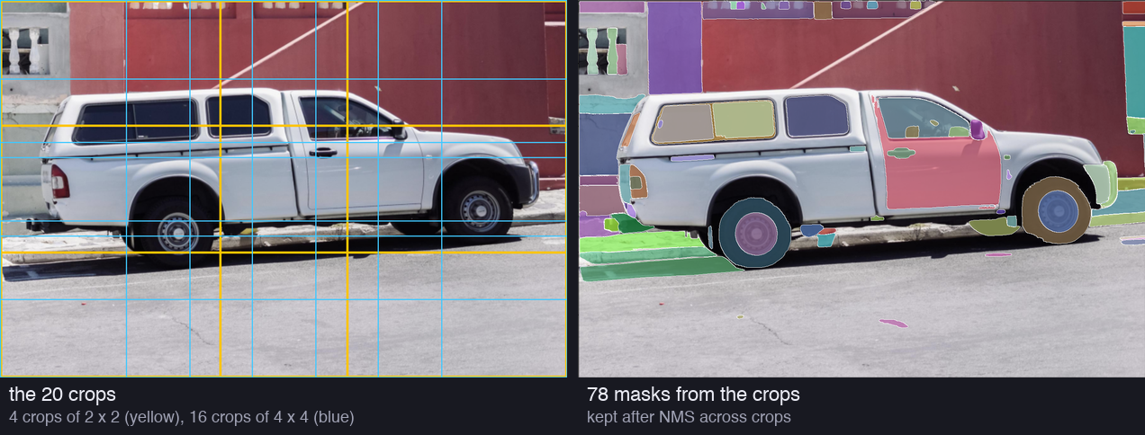
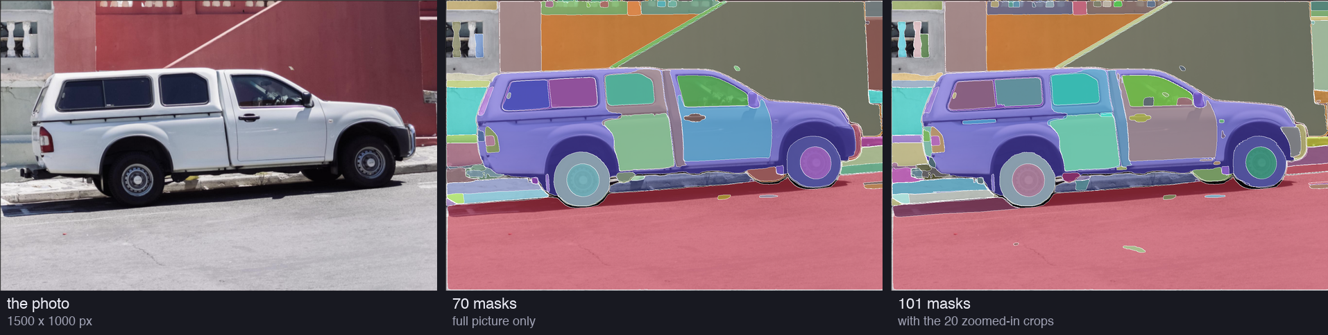
On the car photo, the crops add many small masks. We resized the photo to 1500 × 1000 pixels, the size of the released SA-1B pictures (shortest side 1500). The paper cut its crops from the original high-resolution pictures; we cut ours from the resized photo.
plain text
crops: 21 = 1 full picture + 4 (2 x 2) + 16 (4 x 4); sizes 921 x 671 and 503 x 378 px; points 32 x 32, 16 x 16 and 8 x 8
The 20 crops of the car photo and the 78 masks that survive from them. Each crop is resized to 1024 pixels on its long side before SAM sees it, so small objects become large.
Why does a crop help? SAM always reads a picture at 1024 pixels on its long side. The full photo of 1500 pixels is shrunk to fit, and a crop of 503 pixels is enlarged:
plain text
scale that SAM applies: full car photo 1024 / 1500 = 0.68; a 4 x 4 crop 1024 / 503 = 2.04 -> an object looks 3.0x larger in the crop
A hubcap looks three times larger in a small crop than in the full photo. The 8 × 8 points of the crop also sit closer together on it.
The crops bring one new problem. An object cut by the edge of a crop gives a half mask. So a mask that touches an inner edge of its crop (an edge that is not also an edge of the picture) is removed. When the same object appears in several crops, NMS across crops keeps the mask from the most zoomed-in crop.
plain text
full picture only: 3072 candidates -> IoU 2607 -> stability 1641 -> < 95% 1641 -> NMS 76 -> final 70with crops: 3072 points, 9216 candidates -> IoU 7969 -> stability 5197 -> < 95% 5197 -> not at an inner crop edge 2098 -> NMS in each crop 218 -> NMS across crops 110 -> final 101final masks by source: full picture 23, 2 x 2 crops 33, 4 x 4 crops 45
The car photo with the masks of the fully automatic stage. Middle: 32 × 32 points on the full picture, 70 masks. Right: with the 20 crops, 101 masks.
The crops raise the count from 70 to 101 masks. 78 of the 101 come from crops, and only 23 from the full picture. Our count is close to the "∼100 masks per image" of SA-1B, but that is partly luck. A busy market photo gives many more, and a photo of the sky gives fewer.
The number of masks after each step. The cat photo goes from 3,072 candidates to 23 masks. The car photo with crops goes from 9,216 candidates to 101 masks. NMS removes the most, because so many grid points land on the same object.The 23 final masks of the cat photo, with the 32 × 32 grid on the full picture. Both cats, both remotes, the blanket and parts of the sofa each get one mask; some small parts, such as a tail and paws, get their own.
Does our hand-made version match the library? The transformers library has an automatic mask generator, pipeline("mask-generation"), which follows the released code. It does no clean-up and has no 95% filter, so we compare it with our list before the clean-up:
plain text
pipeline: 30 masks; ours before the clean-up: 30 masks (after it: 23)each of our masks against its best match in the pipeline output: IoU >= 0.99 for 30 of 30, lowest 1.000; pipeline masks with a match >= 0.99 in ours: 30 of 30
The two lists are the same, mask for mask. So the steps above are the whole stage.
What can our run not show? It used the released SAM ViT-H. The masks of SA-1B came from a special model, which the paper describes next and which was not released. Our two photos are also far from the variety of 11 million pictures.
Figure 2 shows what the masks look like. Part 1 showed the whole figure; here are its busiest rows:
plain text
SA-1B pictures: 3300 x 4950 = 16.3M pixels = 53x a COCO picture (480 x 640); released at 1500 x 2250 = 3.38M pixels = 11x COCOgrid spacing on an average SA-1B picture: 103 x 155 px; in the 1024 frame that SAM reads: 32 px
We cannot repeat this study. It needs professional annotators and the SA-1B pictures.
Mask properties: where, how many, how big, what shape#
Two measures need a closer look. The relative size of a mask is
s=picture areamask area
The square root turns an area into a length. A mask that fills a quarter of the picture has s=0.25=0.5: its side is about half the side of the picture. A mask of 1% of the picture has s=0.1.
The concavity of a mask is
c=1−convex hull areamask area
The convex hull is the shape that you get when you stretch a rubber band around the mask. A convex shape, such as a disc or a square, fills its rubber band completely, so c=0. A shape with bays and dents leaves empty space inside the band, so c grows. A tiny example: a 4 × 4 square with a 2 × 2 bite out of one corner. Its area is 12, its hull cuts the corner diagonally and has area 14, so c=1−12/14=0.143.
plain text
tiny example: a 4 x 4 square with a 2 x 2 bite: area 12, convex hull area 14, concavity 1 - 12/14 = 0.143
The legend of Figure 6 gives the size of each dataset. Our script did the divisions:
plain text
dataset sizes (Figure 6 legend): masks per image: SA-1B 103, Open Images 2.7, ADE20K 25, COCO 7.3, LVIS 12.5
  SA-1B / Open Images: images 11x, masks 418x, masks per image 38x; SA-1B / ADE20K masks per image 4.1x (the paper: 3.5x, from exact counts)
With the rounded numbers of the legend, we get 38 times and 4.1 times, where the paper says 36 and 3.5. The paper computed its ratios from exact counts that the legend does not print, so the small gap is rounding.
We can compute the same three properties on our own output. This is a tiny sample, two photos and 130 masks, with crops on both. It is not SA-1B:
plain text
cats: 29 masks; relative size sqrt(area / picture): median 0.057, under 0.1: 20 (69%), 0.1 to 0.3: 6, 0.3 and above: 3 concavity: median 0.101, mean 0.157, max 0.591; under 0.1: 14car: 101 masks; relative size sqrt(area / picture): median 0.039, under 0.1: 83 (82%), 0.1 to 0.3: 14, 0.3 and above: 4 concavity: median 0.049, mean 0.074, max 0.591; under 0.1: 74both photos: 130 masks, 65.0 per photo (SA-1B: 1.1B / 11M = 100 per image); relative size bins 0-0.05-0.1-0.2-0.3-0.5-0.75-1: [72, 31, 17, 3, 4, 3, 0]
Our 130 final masks from two photos. Left: most masks are small, with a relative size under 0.1, as in the SA-1B curve of Figure 6. Right: most masks are almost convex, with a concavity under 0.1.
The pattern is the same as in Figure 6: many small masks, and most of them close to convex. Most masks on the car are windows, wheels, hubcaps and marks on the road. The few concave masks are the cats with their legs out and the blanket around them. Two photos cannot show a distribution of masks per picture; for that, you need thousands of pictures.
The pictures have no GPS tags, so how does the team know the country? Appendix C explains:
The share of images from each region, from Table 1. COCO and Open Images draw almost half of their pictures from North America. SA-1B draws half from Europe and a third from Asia and Oceania. Africa and Latin America stay under 5% in all three.
The paper does not print the masks per image of each group, only the range "94-108". We can compute it from the table:
plain text
Table 1: masks per image in each group = #masks / #images
  Africa                      28M /  0.3M =   93.3;  share of SA-1B images  2.8%  COCO  3.0%  Open Images  1.7%
  Asia & Oceania             423M /  3.9M =  108.5;  share of SA-1B images 36.2%  COCO 11.4%  Open Images 14.3%
  Europe                     540M /  5.4M =  100.0;  share of SA-1B images 49.8%  COCO 34.2%  Open Images 36.2%
  Latin America & Carib.      36M / 0.38M =   94.7;  share of SA-1B images  3.5%  COCO  3.1%  Open Images  5.0%
  North America               80M / 0.83M =   96.4;  share of SA-1B images  7.7%  COCO 48.3%  Open Images 42.8%
  high income                598M /  5.8M =  103.1;  share of SA-1B images 54.0%  COCO 89.1%  Open Images 87.5%
  middle income              499M /  4.9M =  101.8;  share of SA-1B images 45.0%  COCO 10.5%  Open Images 12.0%
  low income                 9.4M /  0.1M =   94.0;  share of SA-1B images  0.9%  COCO  0.4%  Open Images  0.5%
From the rounded table, Africa gives 93.3 masks per image, just under the paper's 94; the exact counts are not printed. The point stands: the engine draws about as many masks on a picture from Lagos as on a picture from Paris. It treats every picture the same way, because no person decides what to label.
The clothing rows come from Appendix C, and they show the one real bias:
Mean IoU with one point and its 95% confidence interval, from Tables 2 and 6. For people, only older and middle age do not overlap. For clothing, feminine (76.3 ± 1.1) and masculine (81.0 ± 1.2) do not overlap: the one bias that the paper reports.
plain text
clothing, gender: gap 81.0 - 76.3 = 4.7 points at 1 point; 92.3 - 90.7 = 1.6 at 3 points; 3-point intervals [90.2, 91.2] and [91.9, 92.7]
Our run cannot test fairness: it would need photos of many people with true masks and group labels. The numbers above are the paper's, and our script only checks the arithmetic.
Appendix F closes the paper's account of the data with three standard documents. They are a dataset card for SA-1B, an annotation card for stages 1 and 2, and a model card for SAM. They answer fixed questions, such as who made the data, what it contains and what it should not be used for. Two answers matter here. The released masks have "no categories or text", and the masks that people drew in stages 1 and 2 "will not be released".
Next, in Part 5: the zero-shot experiments. SAM against other models on 23 datasets, with one click, and on edges, object proposals, instance masks and text.
Run it yourself
The script code/papers/sam/sam_part4.py rebuilds the fully automatic stage by hand. It makes the grid and the three masks of each point and computes the two scores. Then it applies the three filters, greedy NMS, the 20 crops and the clean-up. It checks the result against pipeline("mask-generation") and draws the rejected masks.
It also computes the Section 5 statistics on our two photos and works out the numbers of Tables 1, 2 and 6. Every number of this part is in results/part4.json and results/part4_stdout.txt. The script downloads the car photo from the Hugging Face Hub; it does not download SA-1B.