SAM, explained · Part 3 of 3 · Covers Figure 4, §3, Appendix A, Figure 14

The Model: Encoder, Prompts and Decoder

How SAM turns a photo and a click into three masks and three scores. We open the released model, follow each tensor through it, and compute its training loss by hand.

Segment Anything. Alexander Kirillov, Eric Mintun, Nikhila Ravi, Hanzi Mao, Chloe Rolland, Laura Gustafson, Tete Xiao, Spencer Whitehead, Alexander C. Berg, Wan-Yen Lo, Piotr Dollár, Ross Girshick. ICCV 2023, 2023. arXiv:2304.02643

Part 1 showed what SAM does: a photo and a click go in, and three masks with three scores come out. Now we open the model and follow the numbers through each of its three blocks, with the released weights of SAM ViT-H.

Figure 4: the model in one picture

From the paperFigure 4page 5

What it says

"A heavyweight image encoder outputs an image embedding that can then be efficiently queried by a variety of input prompts to produce object masks at amortized real-time speed. For ambiguous prompts corresponding to more than one object, SAM can output multiple valid masks and associated confidence scores."

What it means

Follow the figure from left to right. The photo goes into the large green box, the image encoder. Out comes the image embedding, drawn as a column of small squares. That column is the summary of the picture that every later step reads.

The key word in the caption is "queried". Think of the embedding as a library that the encoder writes once. Each prompt is a visitor who asks one question: "which pixels belong to the thing at this point?" The visitor does not rewrite the library. It only reads it, so each question is cheap.

Two paths bring the prompt in. Points, boxes and text go through the prompt encoder. A rough mask takes a different path: a small "conv" block, and then a plus sign that adds it to the embedding. At the right end, three masks of the same scissors come out, each with a score. One prompt, several valid answers.

Section 3 names the three components with one adjective each: "an image encoder, a flexible prompt encoder, and a fast mask decoder". The encoder gets no adjective, because it may be slow: it runs once for each picture. Section 3 gives the summary and Appendix A the details, so we read the two together.

The figure below is Figure 4 again, with the real shapes that we measured in the released model. Each number in it comes from our script.

SAM ViT-H with the real shapes. The image encoder runs once: 3 × 1024 × 1024 pixels become 64 × 64 patch vectors of 1,280 numbers, then pass through 32 transformer blocks and a neck, and give the 256 × 64 × 64 image embedding. For each prompt, the prompt encoder makes tokens, and the mask decoder makes three masks of 256 × 256 and three scores.

The image encoder

From the paper§3page 5

What it says

"Motivated by scalability and powerful pre-training methods, we use an MAE [47] pre-trained Vision Transformer (ViT) [33] minimally adapted to process high resolution inputs [62]. The image encoder runs once per image and can be applied prior to prompting the model."

What it means

This sentence packs three choices. The first is the network: a Vision Transformer, which cuts the picture into small squares and treats each square as a word. The second is how it learned before SAM: MAE, a fill-in-the-blanks game on pictures (the yellow boxes below explain both). The third is a change: "minimally adapted to process high resolution inputs".

Why "high resolution"? A standard ViT reads a picture of 224 × 224 pixels. SAM must draw exact edges, so it reads 1024 × 1024 pixels, about 21 times more pixels. The "minimal adaptations" make this possible at a fair cost. Appendix A names them, and we measure them below.

The last sentence is the amortized design of Part 1. "Prior to prompting" means that the encoder can run before the user clicks. In the annotation tool, a server computed the embedding while the annotator looked at the photo.

The encoder is a ViT-H/16. Decode the name: H means "Huge", the largest of the three sizes, and /16 means patches of 16 × 16 pixels. Appendix A gives the details:

From the paper§Apage 16

What it says

The encoder is "a ViT-H/16 with 14×14 windowed attention and four equally-spaced global attention blocks". Its output is "a 16× downscaled embedding of the input image". The team "can afford a high number of image encoder FLOPs because they are computed only once per image, not per prompt".

What it means

"Windowed attention" is the main adaptation. Think of a conference with 4,096 people. If each person must talk to every other person, the conference never ends. So the organisers split the people into small rooms of 14 × 14 = 196 people, and people talk only inside their room. Four times during the day, everybody meets in the main hall. These are the four "global attention blocks".

"16× downscaled" is the patch size again: 1024 / 16 = 64, so the embedding is a grid of 64 × 64 cells. The last sentence gives the reason for the whole design. The encoder may be expensive, because its cost is paid once for each picture and then shared by all the clicks.

Attention, the step that mixes the tokens

Each of the 32 blocks has one attention step. It is the only step in which a token gets information from other tokens, so we read its equation carefully.

Think of a library. Each token writes a short question (its query). Each token also has a label on its spine (its key) and some content inside (its value). A token compares its question with every label. It then takes a mix of the contents, with the most weight on the best matches.

\text{Attention}(Q, K, V) = \text{softmax}\!\left( \frac{Q K^\top}{\sqrt{d}} \right) V

Read it from left to right:

$Q$ , $K$ and $V$ are tables with one row for each token: the queries, the keys and the values. Each row has $d$ numbers. The network makes them from the tokens with three learned matrices.
$Q K^\top$ multiplies each query with each key (a dot product). The result is a table of scores: one score for each pair of tokens. A large score means "this label matches my question".
$\sqrt{d}$ divides the scores to keep them in a moderate range when $d$ is large.
$\text{softmax}$ changes each row of scores into weights that are positive and add up to 1.
The weights multiply $V$ . Each token gets a weighted average of the values: its new information.

A tiny example with $d = 2$ , one query and two keys. Let $q = (1, 0)$ , $k_1 = (2, 0)$ and $k_2 = (0, 2)$ . The scores are $q \cdot k_1 / \sqrt{2} = 1.414$ and $q \cdot k_2 / \sqrt{2} = 0$ . The softmax gives the weights:

\frac{e^{1.414}}{e^{1.414} + e^{0}} = 0.804, \qquad \frac{e^{0}}{e^{1.414} + e^{0}} = 0.196

With the values $v_1 = (10, 0)$ and $v_2 = (0, 10)$ , the output is $0.804 \times (10, 0) + 0.196 \times (0, 10) = (8.04, 1.96)$ . The query matched $k_1$ better, so the output is mostly $v_1$ .

In ViT-H, each block runs 16 copies of this step side by side, the attention heads, each with $d = 80$ and its own matrices. The real cost is in the size of the score table. With global attention, each of the 4,096 tokens compares itself with all 4,096 tokens.

Windowed and global attention

Our script loaded the three released encoders and read their configuration:

plain text

model    blocks  width  heads head dim    MLP  window  global-attention blocks (0-based)
ViT-B        12    768     12       64   3072      14  [2, 5, 8, 11]
ViT-L        24   1024     16       64   4096      14  [5, 11, 17, 23]
ViT-H        32   1280     16       80   5120      14  [7, 15, 23, 31]

All three use windows of 14 × 14 tokens, and all three have exactly four global blocks, spaced evenly. In ViT-H, the global blocks are blocks 8, 16, 24 and 32 (the configuration counts from 0). So the tokens work in their rooms for seven blocks, then meet in the hall once, four times in total.

Why windows of 14 × 14? MAE trained the encoder on pictures of 224 × 224 pixels, which is 14 × 14 patches. A window of 14 × 14 tokens is exactly the view that the encoder knew from pre-training. The paper does not say this, but it is the reason in the ViTDet paper [62] that SAM follows.

There is one small problem: 64 is not a multiple of 14. So each windowed block first pads the grid to 70 × 70 tokens with zeros. It then cuts the grid into 5 × 5 = 25 windows:

plain text

windowed attention: the 64 x 64 grid is padded to 70 x 70 (804 padding cells), then cut into 5 x 5 = 25 windows of 14 x 14 = 196 tokens
  score pairs per head: windowed 25 x 196^2 = 960,400;  global 4096^2 = 16,777,216;  ratio 17.5

Left: the 64 × 64 grid of tokens, padded to 70 × 70 (red strips) and cut into 25 windows of 14 × 14 tokens. One window is highlighted. Right: one global block computes 16,777,216 attention scores per head; one windowed block computes 960,400, 17.5 times fewer. Blocks 8, 16, 24 and 32 of ViT-H are global.

The saving in attention scores is 17.5 times. But attention scores are only part of the work of a block. The MLP and the three matrices that make $Q$ , $K$ and $V$ do the same work in both kinds of block. We counted the FLOPs of one block of each kind:

plain text

one windowed block 176.9 GFLOPs, one global block 248.3 GFLOPs (1.40 x)
  of which attention scores and mixing (2 matrix products, 2 FLOPs per multiply-add): global 4 x 4096^2 x 1280 = 85.9 GFLOPs, windowed 4 x 25 x 196^2 x 1280 = 4.9 GFLOPs
if all 32 blocks were global: 7.96 TFLOPs (1.34 x)

A global block costs 1.4 times a windowed block. With global attention in all 32 blocks, the encoder would need 7.96 TFLOPs in place of 5.96, about 34% more. On the GPU of our laptop, the difference is larger: a global block takes about 2.7 times as long as a windowed block (below). The large table of attention scores also needs much memory.

Windows have a cost: a token in one room cannot see a token in the next room. Think of a cat whose head is in one window and whose tail is in another. The four global blocks fix this. After each global block, every token carries some news from the whole picture back into its room.

We followed one picture through the encoder of ViT-H and printed the shape of the data after each step:

plain text

  pixel values                                     (1, 3, 1024, 1024)          3,145,728 numbers
  patch embedding (16 x 16 conv, stride 16)        (1, 64, 64, 1280)           5,242,880 numbers
  + absolute position embedding                    (1, 64, 64, 1280)           5,242,880 numbers
  windowed block: pad 64 -> 70, cut into windows   (25, 14, 14, 1280)          6,272,000 numbers
  after 32 blocks                                  (1, 64, 64, 1280)           5,242,880 numbers
  neck: 1 x 1 conv 1280 -> 256 + layer norm        (1, 256, 64, 64)            1,048,576 numbers
  neck: 3 x 3 conv 256 -> 256 + layer norm         (1, 256, 64, 64)            1,048,576 numbers
  our step-by-step embedding vs get_image_embeddings: max difference 0.00e+00

The 3 colour numbers of each of the 1024 × 1024 pixels become 4,096 tokens of 1,280 numbers. The encoder adds a learned position vector to each token. Inside a windowed block, the grid becomes 25 separate windows; the extra numbers are the padding. After the 32 blocks, the grid has the same shape as before. But each token now describes its place in the context of the whole picture. Our step-by-step run gives exactly the same embedding as the library function.

The weights of the encoder follow the same plan. Each of the 32 blocks has almost 20 million weights:

plain text

model     patch embed  pos. embed  window block  global block      neck         total
ViT-B         590,592   3,145,728     7,091,328     7,104,128   787,456    89,670,912
ViT-L         787,456   4,194,304    12,599,680    12,612,480   852,992   308,278,272
ViT-H         984,320   5,242,880    19,681,760    19,697,760   918,528   637,026,048
check ViT-H: 984,320 + 5,242,880 + 28 x 19,681,760 + 4 x 19,697,760 + 918,528 = 637,026,048

The 32 blocks hold 98.9% of the encoder's weights. The neck at the end is very small. It is the last part of the encoder:

From the paper§Apage 16

What it says

The input is "1024×1024 obtained by rescaling the image and padding the shorter side". "The image embedding is therefore 64×64." To reduce the channels, SAM uses "a 1×1 convolution to get to 256 channels, followed by a 3×3 convolution also with 256 channels". Each convolution is followed by "a layer normalization".

What it means

Part 1 did the resize and the padding by hand: our 640 × 480 photo became 1024 × 768, plus 256 rows of zeros. The new part is the neck, two small layers after the 32 blocks.

After the blocks, each of the 64 × 64 cells has 1,280 numbers. The 1 × 1 convolution shrinks this to 256 numbers. It applies the same small table of weights at every cell, as one translator who shortens each of 4,096 reports in the same way. The 3 × 3 convolution then lets each cell look at its 8 neighbours, which smooths the grid a little.

Why 256? The decoder works with vectors of 256 numbers. A smaller embedding makes every step of the decoder cheaper, and the decoder runs after every click. So the neck is a gate between the expensive world of the encoder and the cheap world of the decoder.

The prompt encoder

From the paper§3page 5

What it says

There are "two sets of prompts: sparse (points, boxes, text) and dense (masks)". Points and boxes become "positional encodings [95] summed with learned embeddings for each prompt type". Text uses "an off-the-shelf text encoder from CLIP". Masks are "embedded using convolutions and summed element-wise with the image embedding".

What it means

A point is a few numbers: an x, a y and a label. A mask is a whole grid of numbers. So the two kinds of prompt take two different roads. A sparse prompt becomes a few vectors of 256 numbers, the prompt tokens. A dense prompt becomes a grid of the same shape as the image embedding, and the two grids are simply added.

Each point token is a sum of two parts: "where" and "what kind". The positional encoding says where the point is. The learned embedding says what kind of point it is, for example "a point on the object" or "a corner of a box". Think of a parcel label: the address, plus a coloured sticker for "fragile" or "express".

For text, SAM borrows CLIP's text encoder, which already changes a sentence into a vector. The released SAM model does not include this text path. Part 5 shows the text experiment of the paper.

Appendix A gives the exact recipe for points and boxes:

From the paper§Apage 16

What it says

Sparse prompts become "256-dimensional vectorial embeddings". A point is "the sum of a positional encoding [95] of the point's location and one of two learned embeddings" for foreground or background. A box is "an embedding pair": its "top-left corner" and its "bottom-right corner", each with its own learned embedding.

What it means

A point has a label: foreground ("this pixel is part of the object") or background ("this pixel is not"). A background point lets you remove a wrong region, for example a sofa that a mask covered by error. Each label has its own learned vector of 256 numbers.

A box is two points with special labels. The top-left corner gets the learned "top-left" vector, and the bottom-right corner gets the "bottom-right" vector. So a box costs exactly two tokens, the same as one click with its padding token (below). The decoder never sees a rectangle. It sees two labelled points and learns what they mean.

The positional encoding of a click

How do you change a position, two numbers, into 256 numbers that a network can use? SAM uses random Fourier features, from the paper cited as [95] (Tancik et al., 2020).

Here is the idea. Lay many striped patterns over the picture, like zebra stripes, each at its own angle and width. For each pattern, write down where the point falls inside its stripe: at the start, the middle or the end. One pattern alone does not identify the point, because the stripes repeat. But many patterns together give a code that differs for every place. It works like a clock with many hands at different speeds: the set of all hand positions tells the exact time.

The formula is:

\gamma(\mathbf{c}) = \Big[ \sin\!\big(2\pi\, \mathbf{c}^\top G\big), \; \cos\!\big(2\pi\, \mathbf{c}^\top G\big) \Big], \qquad \mathbf{c} = (2u - 1, \; 2v - 1)

Read it from right to left this time:

$u$ and $v$ are the position of the point as fractions of the 1024 × 1024 square. They go from 0 at the left or top edge to 1 at the right or bottom edge. $\mathbf{c}$ moves them to the range from $-1$ to $+1$ .
$G$ is a table of 2 rows and 128 columns. Each column $\mathbf{g}$ is one striped pattern: its direction and its number of stripes. The numbers of $G$ are random. They are drawn once, before training, and never change.
$\mathbf{c}^\top G$ multiplies the point with each column: 128 numbers. Each one says "how far along this pattern" the point is.
$2\pi$ changes "how far" into an angle, and $\sin$ and $\cos$ give the position inside the stripe.
$\gamma(\mathbf{c})$ joins the 128 sines and the 128 cosines: 256 numbers.

A tiny example in one dimension with one pattern, $g = 3$ . The angle is $2\pi \times 3 \times x$ :

point $x$	angle	$(\sin, \cos)$
0.10	1.885	(+0.951, −0.309)
0.12	2.262	(+0.771, −0.637)
0.30	5.655	(−0.588, +0.809)

The two near points get similar pairs. The far point gets a very different pair. This is what we want from a code for positions.

Now the real click on the cat's ear, at pixel (275, 62) of the photo. Our script follows it through each step:

plain text

random matrix G: shape (2, 128), mean -0.100, std 1.043  (drawn once at random, then kept fixed)
click (275, 62) in the photo -> x 1.6 -> (440.0, 99.2) in the 1024 frame -> +0.5 (pixel centre) / 1024 -> (0.4302, 0.0974) -> 2u - 1 -> (-0.1396, -0.8053)
  column 0: g = (-0.483, +1.120);  c . g = -0.1396 x -0.483 + -0.8053 x +1.120 = -0.8343;  angle 2 pi x -0.8343 = -5.242;  sin +0.863, cos +0.505
  column 1: g = (-0.663, -0.098);  c . g = -0.1396 x -0.663 + -0.8053 x -0.098 = +0.1717;  angle 2 pi x +0.1717 = +1.079;  sin +0.881, cos +0.472
  column 2: g = (+0.062, -0.613);  c . g = -0.1396 x +0.062 + -0.8053 x -0.613 = +0.4848;  angle 2 pi x +0.4848 = +3.046;  sin +0.095, cos -0.995
positional encoding: 128 sines + 128 cosines = 256 numbers; first four: +0.863, +0.881, +0.095, +0.977
stripe width (period) of each of the 128 frequencies, in pixels of the 1024 frame: shortest 157.8, median 400.1, longest 5188

The click is first scaled by 1.6, as in Part 1, to $(440.0, 99.2)$ . SAM adds 0.5 to aim at the centre of the pixel and divides by 1024. That gives $(u, v) = (0.4302, 0.0974)$ , and then $\mathbf{c} = (-0.1396, -0.8053)$ . For the first column of $G$ :

\mathbf{c} \cdot \mathbf{g}_0 = (-0.1396)(-0.483) + (-0.8053)(1.120) = -0.8343, \qquad \sin(2\pi \times -0.8343) = 0.863

The stripes have widths from 158 to 5,188 pixels. The narrow stripes separate places that are close together. The wide stripes tell the left half of the picture from the right half. So the code is exact at small scales and at large scales.

Does the code behave as promised? We compared the code of the click with the code of every cell of the 64 × 64 grid:

The cosine similarity between the code of the click and the code of each place of the photo. It is 0.999 at the click, 0.979 one cell (16 pixels) away, 0.701 four cells away and −0.016 sixteen cells away. Near places have similar codes; far places have unrelated codes.

The same table $G$ also makes the codes of the 64 × 64 cells of the image embedding. So a click and the cell under it get almost the same code, and the decoder can match them. This shared table is the bridge between the prompt and the picture.

The script then compared our hand-made code with the model's own prompt tokens:

plain text

sparse prompt embedding from the model: (1, 1, 2, 256)  (image, prompts, tokens, 256): the click + one padding token
  token 1 = positional encoding + learned "foreground point" vector: max difference to ours 2.38e-07
  token 2 = the learned "not a point" vector (padding): max difference 0.00e+00
dense prompt embedding (no mask given): (1, 256, 64, 64): one learned "no mask" vector copied to all 64 x 64 cells

The first token is our positional code plus the learned "foreground point" vector, to the seventh decimal place. The second token is a surprise. With a click and no box, SAM adds a padding token: a learned "not a point" vector. The original code pads point prompts in this way when no box is present. It keeps the input in the shape that the decoder saw in training.

Masks as prompts

From the paper§Apage 16

What it says

Masks enter "at a 4× lower resolution than the input image". Then "two 2×2, stride-2 convolutions with output channels 4 and 16" and "a final 1×1 convolution maps the channel dimension to 256". The result and the image embedding "are then added element-wise". With no mask prompt, "a learned embedding representing 'no mask'" is added to each place.

What it means

A mask prompt is usually SAM's own earlier answer: the 256 × 256 mask from the last click. The convolutions shrink it to the 64 × 64 grid of the image embedding, and make 256 numbers at each cell. Then SAM adds the two grids, cell by cell, as you add two photos on a light table.

The "no mask" case is a clever detail. The decoder always gets the sum of two grids, so it never has to ask "is there a mask prompt?". When there is none, the second grid is the same learned vector at every cell. Training taught the decoder to read this neutral signal as "no mask".

Our run shows the shapes:

plain text

mask prompt 256 x 256: conv 2x2 stride 2 -> (1, 4, 128, 128); conv 2x2 stride 2 -> (1, 16, 64, 64); conv 1x1 -> (1, 256, 64, 64); then added to the image embedding cell by cell
weights of the prompt encoder: random matrix G (2 x 128) 256, point and corner types (4 x 256) 1,024, "not a point" (256) 256, "no mask" (256) 256, mask convolutions 4,684; total 6,476

That is the whole prompt encoder: 6,476 numbers, and 256 of them are the random table $G$ . Part 1 counted the same total. A single block of the image encoder has about 3,000 times more weights.

The mask decoder

From the paper§3page 5

What it says

The decoder maps "the image embedding, prompt embeddings, and an output token to a mask". It is "a modification of a Transformer decoder block followed by a dynamic mask prediction head". The block uses "cross-attention in two directions (prompt-to-image embedding and vice-versa)". At the end, "an MLP maps the output token to a dynamic linear classifier, which then computes the mask foreground probability at each image location".

What it means

The decoder has a strange job. Its inputs are a few tokens and a large grid, and its output is a picture-sized mask. The paragraph gives the plan in three steps.

First, the tokens and the image talk to each other, in both directions, for two rounds. Second, the image grid is made larger again. Third, a special token, the "output token", turns into a small filter. The filter is applied at every pixel, and the result is the mask.

"Dynamic linear classifier" is the clever part. A normal classifier has fixed weights after training. Here the weights of the last layer are computed for each prompt, from the output token. A click on an ear makes an "ear detector"; a click on a remote makes a "remote detector". The same decoder can draw any object, because it builds the right detector on the fly.

Appendix A draws the decoder in Figure 14:

From the paperFigure 14page 16

What it says

"A two-layer decoder updates both the image embedding and prompt tokens via cross-attention. Then the image embedding is upscaled, from which the updated output tokens are used to dynamically predict masks." At every attention layer, "positional encodings are added to the image embedding, and the entire original prompt token (including position encoding) is re-added to the token queries and keys".

What it means

Read the figure as two lanes. The top lane carries the image embedding, 256 × 64 × 64. The bottom lane carries the tokens. The darker box in the middle is one decoder layer, and "x2" says that SAM runs it two times.

On the right, the lanes separate. The image lane goes up through "2x conv. trans.", which makes the grid larger. The token lane meets the image once more, then splits. Each mask token goes through its own MLP and meets the large grid in a "dot product per mask". The IoU token goes through a different MLP and gives the scores.

Before we read the four steps, we need the word "token" in its exact meaning here:

From the paper§Apage 16

What it says

Before the decoder runs, SAM inserts "a learned output token embedding that will be used at the decoder's output, analogous to the [class] token in [33]". The prompt embeddings and the output tokens together are the "tokens".

What it means

An output token is an empty notebook that SAM sends into the meeting. It carries no information about this picture at the start: it is the same learned vector for every picture and every click. During the decoder, it collects information from the prompt tokens and from the image. At the end, SAM reads the notebook and draws the mask from it.

ViT uses the same trick for classification: an extra [class] token collects a summary of the picture, and the classifier reads only that token. SAM has five such notebooks: one for the IoU scores and four for masks.

Our run lists the tokens that enter the decoder for the click on the ear:

plain text

tokens: 5 output tokens (1 IoU + 4 mask) + 2 prompt tokens = (1, 7, 256)
image: embedding + dense prompt, flattened: (1, 4096, 256)  (the 64 x 64 grid as 4,096 vectors)

Seven tokens on one side, 4,096 image vectors on the other side. Now the four steps:

From the paper§Apage 16

What it says

Each decoder layer performs four steps: "(1) self-attention on the tokens, (2) cross-attention from tokens (as queries) to the image embedding, (3) a point-wise MLP updates each token, and (4) cross-attention from the image embedding (as queries) to tokens". Each step has "a residual connection, layer normalization, and a dropout of 0.1 at training". "We use a two-layer decoder."

What it means

Picture a meeting between seven detectives (the tokens) and a wall of 4,096 photos (the image vectors). Each step is one part of the meeting:

The detectives talk to each other (self-attention). The output tokens learn where the click is and what kind of click it is.
The detectives look at the wall (token-to-image attention). Each token asks a question, and the image vectors answer. The mask tokens collect what the image looks like near the click.
Each detective thinks alone (MLP). Each token passes through a small network by itself, with no exchange.
The wall looks at the detectives (image-to-token attention). Now the image vectors ask, and the tokens answer. Each image vector learns about the prompt: "someone clicked on an ear near here".

Step 4 is the new idea, and it gives the name "two-way". A standard transformer decoder only lets the tokens read the image. SAM also lets the image read the tokens. So after two layers, the image grid itself knows about the click, and the final dot product can use that knowledge at every pixel.

One layer of the mask decoder. Steps 1 to 3 update the 7 tokens: they talk to each other, read the 4,096 image vectors, and each passes through an MLP. Step 4 updates the image: each image vector reads the tokens. The decoder runs this layer two times.

To check that we understand the four steps, we wrote the decoder again by hand, with the model's own weights. Then we compared our result with the model's output. The core is a few lines:

python

def attend(mod, q, k, v):      # SAM's attention: project, 8 heads, softmax(q k^T / sqrt(d)) v, join, project
    Q, K, V = mod.q_proj(q), mod.k_proj(k), mod.v_proj(v)
    ...
for L in decoder.transformer.layers:                     # two layers
    q = L.layer_norm1(q + attend(L.self_attn, q + tokens, q + tokens, q))                            # step 1
    q = L.layer_norm2(q + attend(L.cross_attn_token_to_image, q + tokens, keys + kpe, keys))         # step 2
    q = L.layer_norm3(q + L.mlp(q))                                                                  # step 3
    keys = L.layer_norm4(keys + attend(L.cross_attn_image_to_token, keys + kpe, q + tokens, q))      # step 4

Here q is the 7 tokens and keys is the 4,096 image vectors. tokens is the original tokens, and kpe is the positional code of each image cell. (In the first layer, step 1 has no residual and no added code; the script handles this case.) The output:

plain text

  layer 1, step 1: self-attention among the 7 tokens         (1, 7, 256)
  layer 1, step 2: tokens attend to the 4,096 image vectors  (1, 7, 256)
  layer 1, step 3: MLP on each token                         (1, 7, 256)
  layer 1, step 4: image vectors attend to the tokens        (1, 4096, 256)
  layer 2, step 1: self-attention among the 7 tokens         (1, 7, 256)
  layer 2, step 2: tokens attend to the 4,096 image vectors  (1, 7, 256)
  layer 2, step 3: MLP on each token                         (1, 7, 256)
  layer 2, step 4: image vectors attend to the tokens        (1, 4096, 256)
  final: tokens attend to the image once more                (1, 7, 256)
  upscale: transposed conv 2x2, stride 2                     (1, 64, 128, 128)
  upscale: transposed conv 2x2, stride 2                     (1, 32, 256, 256)
  4 mask tokens through their MLPs                           (1, 4, 32)
  dot product with every pixel vector -> 4 masks             (1, 4, 256, 256)
  IoU token through the IoU head -> 4 scores                 (1, 4)
our hand-written decoder vs the model: masks max difference 3.66e-04, scores max difference 1.19e-07

Our masks agree with the model's masks to 0.0004, on mask values that range up to about 34. The small difference comes from the order of the GPU's additions. So the four steps in the paper are the whole decoder.

Look at the code again. Every attention call adds tokens to the token side and kpe to the image side. The paper explains why:

From the paper§Apage 16

What it says

"the positional encodings are added to the image embedding whenever they participate in an attention layer". Also, "the entire original prompt tokens (including their positional encodings) are re-added to the updated tokens". This "allows for a strong dependence on both the prompt token's geometric location and type".

What it means

Attention by itself has no sense of place. It treats the 4,096 image vectors as a bag, with no order. If the positions go in only once, at the start, the decoder can lose them as the vectors change from step to step.

So SAM pins the address on again before every attention step. The image vectors get their cell codes, and the tokens get their original values, with the click's code inside. Think of a guide who repeats "we are at the ear" before every question. The answer can never drift away from the place of the click.

We counted the weights of each piece of the decoder:

plain text

weights of the mask decoder:
  output tokens (1 IoU + 4 mask, x 256)           1,280
  two-way layer 1                             1,579,520
  two-way layer 2                             1,579,520
  final token-to-image attention + norm         132,224
  upscaling (2 transposed convs + norm)          73,952
  4 mask MLPs (256 -> 256 -> 256 -> 32)         559,232
  IoU head (256 -> 256 -> 256 -> 4)             132,612
  total                                       4,058,340
  inside one two-way layer: self-attention 263,168, token-to-image attention 131,712, MLP 256 -> 2048 -> 256 1,050,880, image-to-token attention 131,712, 4 layer norms 2,048
attention widths: self-attention q, k, v = 256 (8 heads of 32); cross-attention q, k, v = 128 (8 heads of 16)

Appendix A gives the sizes behind these counts: width 256, an MLP of 2,048 numbers inside, and 8 heads in each attention. The MLP holds two thirds of each layer's weights, but it touches only the 7 tokens, so it is cheap. The two cross-attentions touch all 4,096 image vectors, so the team halved their width to 128. The whole decoder, 4.06 million weights, is smaller than one block of the image encoder (19.7 million).

From tokens to a mask

After the two layers, the decoder has 7 updated tokens and an updated 64 × 64 grid. One cell of the grid covers 16 × 16 pixels, which is too coarse for an exact edge. So the decoder first makes the grid larger:

From the paper§Apage 16

What it says

SAM upsamples "the updated image embedding by 4×" with two transposed convolutions, "2×2, stride 2 with output channel dimensions of 64 and 32". Then "the tokens attend once more to the image embedding". Each output token goes through "a small 3-layer MLP". The mask is "a spatially point-wise product between the upscaled image embedding and the MLP's output".

What it means

Each transposed convolution doubles the width and the height of the grid: 64 to 128 to 256. At the same time, it reduces the numbers at each cell: 256 to 64 to 32. So the decoder trades depth for detail. Each pixel of the 256 × 256 grid gets a short description of 32 numbers.

The mask token goes through its own small MLP and becomes 32 numbers too. Now the two sides have the same length, and SAM takes their dot product at every one of the 65,536 places. The result is one number at each place: the mask, at a quarter of the 1024 × 1024 input size. Part 1 scaled these 256 × 256 masks back to our 640 × 480 photo.

The dot product is the "dynamic linear classifier" of §3. Here is its equation, for mask $k$ at pixel $(i, j)$ :

m_k(i, j) = \mathbf{w}_k \cdot \mathbf{f}(i, j) = \sum_{c=1}^{32} w_{k,c} \, f_c(i, j), \qquad p_k(i, j) = \sigma\big(m_k(i, j)\big) = \frac{1}{1 + e^{-m_k(i, j)}}

Think of a paint-matching card. The mask token describes the object that the user wants, as 32 numbers: the card. Each pixel has its own description, also 32 numbers. At each pixel, SAM holds the card next to the pixel and asks "how well do they match?". The dot product is that match.

Read it from left to right:

$m_k(i, j)$ is the raw score of mask $k$ at pixel $(i, j)$ , the logit. Positive means "inside", negative means "outside".
$\mathbf{w}_k$ is the card: the 32 numbers that the MLP made from mask token $k$ . It is the same at all pixels, and it changes with the prompt.
$\mathbf{f}(i, j)$ is the description of the pixel: the 32 numbers of the upscaled grid. It is the same for all masks.
The sum multiplies the 32 pairs and adds the products.
$\sigma$ , the sigmoid, changes the logit into a probability between 0 and 1. A logit of 0 gives 0.5.

A tiny example with 3 numbers in place of 32. Let the card be $\mathbf{w} = (2, -1, 0.5)$ . A pixel with $\mathbf{f} = (0.3, 0.2, 0.4)$ gets $m = 0.6 - 0.2 + 0.2 = 0.6$ , so $p = \sigma(0.6) = 0.646$ : probably inside. A pixel with $\mathbf{f} = (-0.1, 0.5, 0)$ gets $m = -0.2 - 0.5 + 0 = -0.7$ , so $p = 0.332$ : probably outside.

Now the real numbers from the ear click, at three pixels of the photo:

plain text

the dynamic dot product: mask logit at pixel = (32 numbers from the mask token) . (32 numbers of the upscaled pixel)
  mask token 1, first 4 numbers w = -139.524, -5.909, -194.530, +5.933;  pixel at the ear, first 4 numbers f = -0.053, +0.129, -0.145, +0.372
  the 3 largest products w_i f_i: i=20: +278.544 x +0.109 = +30.370, i=2: -194.530 x -0.145 = +28.284, i=13: +191.332 x +0.139 = +26.634
  ear       photo (275, 62)   -> 256 grid (110,  24):  mask 1 (ear) logit  +33.97 -> p 1.000;   mask 3 (cat) logit   +9.90 -> p 1.000
  cat body  photo (120, 220)  -> 256 grid ( 48,  88):  mask 1 (ear) logit  -22.51 -> p 0.000;   mask 3 (cat) logit   +4.14 -> p 0.984
  blanket   photo (250, 400)  -> 256 grid (100, 160):  mask 1 (ear) logit  -35.86 -> p 0.000;   mask 3 (cat) logit  -10.85 -> p 0.000

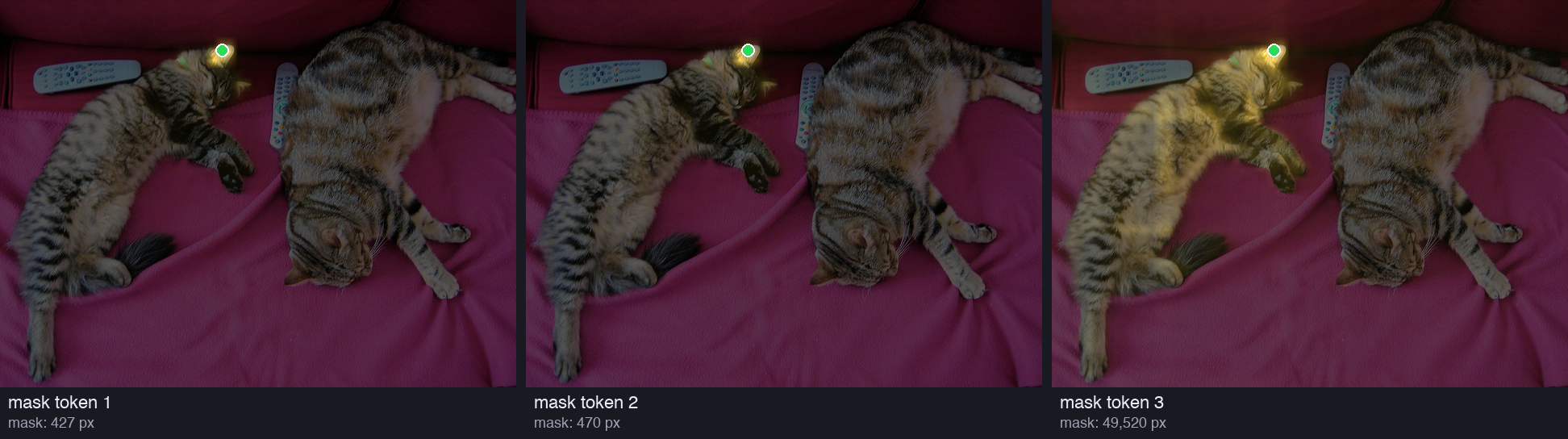
The dynamic dot product at three pixels. At the ear, both the ear mask and the cat mask are positive. On the cat's body, only the cat mask is positive (+4.14). On the blanket, both are negative. The pixel descriptions are the same for every mask; only the 32 numbers of the mask token change.

The table reads like a sentence. At the ear, both cards match: the ear is part of the ear and part of the cat. On the body, the ear card says "no" (−22.51) and the cat card says "yes" (+4.14). On the blanket, both cards say "no". The pixel descriptions did not change between the two masks. Only the card changed.

The card's numbers are large (−139.5, −194.5) and the pixel numbers are small (−0.053, −0.145). Their products are large: the three largest products alone add up to more than 85. So the logits are far from 0 at most pixels, and the sigmoid gives almost exactly 0 or 1. The uncertain pixels are only near the edges.

Where do the mask tokens look? The last token-to-image attention shows it. We averaged its 8 heads for each mask token:

Three dark copies of the photo, each with a bright heat map. For mask tokens 1 and 2, a small bright spot sits on the left cat's ear, at the click. For mask token 3, a weaker glow spreads over the head and the body of the left cat — The final token-to-image attention of the three mask tokens, averaged over the 8 heads (brighter = more attention, square-root scale). The ear tokens 1 and 2 put up to 0.217 of their attention on one cell near the click. The cat token 3 spreads its attention: its strongest cell gets only 0.023.

The ear tokens look at one small place. The cat token spreads its attention over the cat, because its answer is large. Nobody told the tokens to do this. Training discovered it.

Resolving ambiguity

From the paper§3page 5

What it says

"With one output, the model will average multiple valid masks if given an ambiguous prompt." So SAM predicts several masks, and "3 mask outputs is sufficient to address most common cases (nested masks are often at most three deep: whole, part, and subpart)". "During training, we backprop only the minimum loss [15, 45, 64] over masks." A confidence score, the "estimated IoU", ranks the masks.

What it means

Imagine a student who must answer "what does this click mean?" with one drawing. Half of the time, the teacher wanted the ear; the other half, the cat. The safest single drawing is a blur: the ear in full, and the cat at half strength. That blur matches no answer well. This is "average multiple valid masks".

The fix is to let the student give three drawings, and to grade only the best one. Now the student can draw the ear in one slot and the cat in another, and neither drawing is punished for the other meaning. Why three? Objects nest: a whole (the cat), a part (the head), a subpart (the ear). Three levels cover most clicks.

"Backprop" is short for backpropagation, the step that computes how to change each weight. "Only the minimum" means that the two other masks get no correction from this example at all.

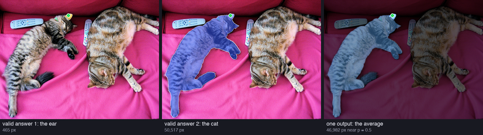
We can see the blur with real numbers. Take two valid answers for the ear click: "the ear" and "the cat". Average SAM's probabilities for its ear mask and its cat mask, as a single-output model would learn to do:

Three panels. Left: a small yellow mask on the cat's ear, 465 pixels. Middle: a blue mask over the whole left cat, 50,517 pixels. Right: a dark photo where the ear is bright and the whole cat glows at half strength, 46,982 pixels near probability 0.5 — Two valid answers for one click, and their average. The average is sure about the ear but unsure about the rest of the cat: 46,982 pixels have a probability between 0.4 and 0.6.

plain text

one output that averages "ear" and "cat" (probability 0.5 on the cat body):
  against the ear: mask loss 1.3399  (best of the three masks: 0.0152)
  against the cat: mask loss 0.5388  (best of the three masks: 0.0471)
  pixels with a probability between 0.4 and 0.6: 46,982 (a blurred, unsure mask)

The averaged mask is bad for both meanings. Its loss (defined below) is 88 times the best of SAM's three masks if the user wanted the ear. It is 11 times worse if the user wanted the cat. Three outputs remove the problem.

Appendix A gives the details:

From the paper§Apage 17

What it says

SAM uses "a small number of output tokens and predict[s] multiple masks simultaneously". It computes the loss for each mask, "but only backpropagate[s] from the lowest loss". A small head on "an additional output token" "estimates the IoU between each predicted mask and the object it covers".

What it means

One output token gives one mask, so three masks need three mask tokens. The tokens start as three different learned vectors. Training then pushes them apart: each one becomes good at one level of the nest. In our runs, token 3 gave the largest mask. It gave the whole cat here, and a large region of the sofa for the remote click of Part 1.

The IoU head is a fourth kind of notebook: it does not draw a mask, it grades the masks. It answers "how good is each of my three masks?". The user has no correct mask at prediction time, so the model must estimate the score by itself. These are the scores of Part 1.

And one more detail explains the strange fourth mask token:

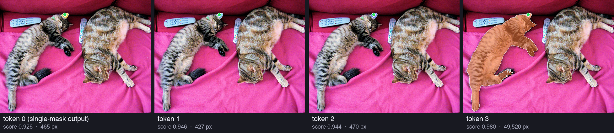
We printed all four masks for the single ear click:

plain text

the four mask tokens for the single ear click (token 0 is the single-mask output for several prompts):
  token 0: predicted IoU 0.926       465 pixels
  token 1: predicted IoU 0.946       427 pixels
  token 2: predicted IoU 0.944       470 pixels
  token 3: predicted IoU 0.980    49,520 pixels

Four copies of the photo with the click on the ear. Token 0, token 1 and token 2 each show a small mask on the ear, of 465, 427 and 470 pixels. Token 3 shows an orange mask over the whole left cat, 49,520 pixels — All four mask tokens for the one click on the ear. Tokens 1 to 3 are the three masks that SAM returns for one click. Token 0 is the single-mask slot for several clicks; for one click, it gives the ear (465 pixels).

Token 0 chose the ear. Training uses this token for several prompts, so SAM does not return it for one click. Tokens 1, 2 and 3 are the masks that Part 1 showed.

Efficiency

We counted the operations of each part and timed them on our laptop:

plain text

image encoder ViT-H: 5.96 TFLOPs per picture
prompt encoder + mask decoder: 3.62 GFLOPs per prompt = 0.06% of the encoder
MPS  image encoder  2999.4 ms  (patch embed 7.0, windowed block 81.9, global block 217.5, neck 2.7)   prompt encoder 0.40 ms   mask decoder 6.02 ms   both 6.49 ms
CPU  image encoder  6779.2 ms  (patch embed 19.2, windowed block 245.7, global block 358.0, neck 8.7)   prompt encoder 0.05 ms   mask decoder 14.44 ms   both 15.82 ms

Top: the work for one picture and one click. The image encoder needs 5.96 trillion operations; the prompt encoder and the mask decoder need 3.62 billion, 0.06% of the encoder. Bottom: on the laptop GPU, almost all the time goes to the 32 blocks of the encoder.

The encoder does about 1,650 times more work than the decoder. Appendix A says that the decoder "requires less than 1% of the image encoder's compute"; our count gives 0.06%, so "less than 1%" is modest. On the CPU, the prompt encoder and the decoder together take 16 ms, well under the paper's 50 ms in a browser.

Look inside the encoder's time. A windowed block takes 82 ms on the GPU, and a global block takes 218 ms. The four global blocks are one eighth of the blocks, but they take more than a quarter of the encoder's time. With 32 global blocks, the encoder would be more than twice as slow on this computer.

The losses

From the paper§Apage 17

What it says

"a 20:1 ratio of focal loss to dice loss". "Auxiliary deep supervision after each decoder layer is unhelpful." The IoU head is trained "with mean-square-error loss between the IoU prediction and the predicted mask's IoU with the ground truth mask", added "with a constant scaling factor of 1.0".

What it means

There are three parts. Focal loss grades each pixel. Dice loss grades the overlap of the whole mask. The squared error grades the IoU head. The focal loss gets 20 times the weight of the dice loss, because it is usually a much smaller number (we see this below).

"Auxiliary deep supervision" means extra losses in the middle of a network, for example a mask after decoder layer 1 as well as after layer 2. The models that SAM borrows from, DETR [14] and MaskFormer [20], do this. SAM tried it and found no gain. With only two layers, there is little "middle" to supervise.

The Background page gave this loss in short. Now we take each part in turn, and then compute all of it on SAM's real masks.

We need a correct mask for that. Our photo has no hand-drawn mask, so we made two stand-in references with SAM itself, from box prompts. "The ear" is SAM's mask for a tight box around the ear (465 pixels). "The cat" is SAM's mask for a box around the left cat (50,517 pixels). The masks that we grade are the three masks of the single ear click.

Focal loss: grade the hard pixels

Most pixels are easy. For our ear click, more than 99% of the photo is clearly "not the ear". Plain cross-entropy charges a small amount for each of these easy pixels, and hundreds of thousands of small amounts add up. The few hard pixels at the edge, where the model is really unsure, get lost in the crowd. Focal loss turns down the easy pixels.

\text{FL}(p_t) = -\alpha_t \, (1 - p_t)^{\gamma} \log p_t, \qquad p_t = \begin{cases} p & \text{if } y = 1 \\ 1 - p & \text{if } y = 0 \end{cases}

Read it from the right:

$p$ is the probability that SAM gives to "inside" at one pixel, and $y$ is the correct answer (1 inside, 0 outside). $p_t$ is the probability of the correct answer. If the pixel is outside and $p = 0.2$ , then $p_t = 0.8$ .
$-\log p_t$ is the cross-entropy of the Background page: near 0 when $p_t$ is near 1, and large when $p_t$ is small.
$(1 - p_t)^{\gamma}$ is the new factor, with $\gamma = 2$ . For an easy pixel, $p_t$ is near 1, so the factor is near 0. For a hard pixel, the factor is near 1.
$\alpha_t$ is a fixed weight for the two classes: $\alpha = 0.25$ for "inside" pixels and $1 - \alpha = 0.75$ for "outside" pixels. The paper does not give $\alpha$ or $\gamma$ . We use $\gamma = 2$ and $\alpha = 0.25$ , the values of the focal-loss paper [65] and of the code that SAM follows.
The loss of the mask is the average over all pixels.

Three pixels show the effect:

pixel	$p_t$	cross-entropy $-\log p_t$	$(1 - p_t)^2$	focal loss
easy, inside, $p = 0.9$	0.9	0.1054	0.0100	$0.25 \times 0.0100 \times 0.1054 = 0.00026$
hard, inside, $p = 0.3$	0.3	1.2040	0.4900	$0.25 \times 0.4900 \times 1.2040 = 0.14749$
wrong, outside, $p = 0.6$	0.4	0.9163	0.3600	$0.75 \times 0.3600 \times 0.9163 = 0.24740$

In cross-entropy, the hard pixel costs 11 times the easy one. In focal loss, it costs about 560 times as much. The easy pixel almost disappears from the sum.

The loss of one pixel against p_t, the probability that the model gives to the correct answer (without the factor α). Cross-entropy still charges about 0.1 at p_t = 90%. Focal loss charges almost nothing once p_t is above 70%, and keeps most of the penalty for the hard pixels on the left.

Dice loss: grade the overlap

Focal loss looks at one pixel at a time. It does not care about the size of the object. A small ear of 465 pixels is less than 0.2% of the 307,200 pixels of the photo. So even a missing ear changes the average focal loss very little. Dice loss looks at the whole mask at once.

L_{\text{dice}} = 1 - \frac{2 \sum_{i} p_i \, y_i + 1}{\sum_{i} p_i + \sum_{i} y_i + 1}

Read it from the inside:

$\sum_i p_i y_i$ adds the probabilities at the pixels that are truly inside. It is a soft version of the overlap $|A \cap B|$ of Part 1.
$\sum_i p_i + \sum_i y_i$ is the soft size of the predicted mask plus the size of the correct mask.
The fraction is the dice score. It is 1 for a perfect mask and 0 for no overlap. It is a close relative of IoU: $2|A \cap B| / (|A| + |B|)$ .
The "+1" on the top and the bottom keeps the fraction defined when both masks are empty.
$1 -$ the score changes "good" into "loss".

A tiny example with 4 pixels: $p = (0.9, 0.8, 0.3, 0.1)$ and $y = (1, 1, 1, 0)$ . Without the +1:

\text{dice} = \frac{2 \times (0.9 + 0.8 + 0.3)}{(0.9 + 0.8 + 0.3 + 0.1) + 3} = \frac{4.0}{5.1} = 0.7843, \qquad L_{\text{dice}} = 0.2157

The dice loss does not depend on the size of the picture. A mask that misses half of a small ear loses about half of its dice score. A mask that misses half of a cat loses the same. So dice loss protects the small objects, and focal loss sharpens the edges.

The IoU head: grade the grader

L_{\text{IoU}} = \big( \hat{s} - \text{IoU}(M, Y) \big)^2

$\hat{s}$ is the score that the IoU head predicts for mask $M$ . $\text{IoU}(M, Y)$ is the real IoU of $M$ with the correct mask $Y$ , after the threshold at $p = 0.5$ . The square of the difference is the mean squared error: a predicted 0.90 for a real IoU of 0.80 costs $(0.90 - 0.80)^2 = 0.0100$ .

All together: the minimum over three masks

Put the parts together. For one prompt with the three masks $M_1, M_2, M_3$ , scores $\hat{s}_1, \hat{s}_2, \hat{s}_3$ and correct mask $Y$ :

L = \min_{k \in \{1, 2, 3\}} \Big[ 20 \, \text{FL}(M_k, Y) + L_{\text{dice}}(M_k, Y) \Big] \; + \; 1.0 \cdot \frac{1}{3} \sum_{k=1}^{3} \big( \hat{s}_k - \text{IoU}(M_k, Y) \big)^2

The first part is the mask loss of the best mask only. The second part grades the IoU head. The paper does not say whether the IoU term uses all three masks or only the best one. We take the average of all three, because the head must score every mask that it returns.

Now the real numbers. The same three masks, graded against the two references:

plain text

target: the ear
  mask    pixels    focal  20 x focal    dice  mask loss  true IoU  pred. IoU  (pred - true)^2  CE (for comparison)
  1          427   0.0001      0.0027  0.0472     0.0498     0.914      0.946           0.0010               0.0006
  2          470   0.0000      0.0006  0.0145     0.0152     0.981      0.944           0.0013               0.0001
  3       49,520   0.4899      9.7974  0.9820    10.7793     0.009      0.980           0.9431               0.6826
  the minimum mask loss is mask 2: 0.0152. Only mask 2 gets a gradient from the mask loss.
  IoU term (mean over the 3 masks): 0.3152;  total = 0.0152 + 1.0 x 0.3152 = 0.3303
target: the cat
  mask    pixels    focal  20 x focal    dice  mask loss  true IoU  pred. IoU  (pred - true)^2  CE (for comparison)
  1          427   1.0322     20.6436  0.9839    21.6275     0.008      0.946           0.8804               4.1283
  2          470   0.9960     19.9192  0.9819    20.9011     0.009      0.944           0.8750               3.9836
  3       49,520   0.0008      0.0157  0.0314     0.0471     0.976      0.980           0.0000               0.0128
  the minimum mask loss is mask 3: 0.0471. Only mask 3 gets a gradient from the mask loss.
  IoU term (mean over the 3 masks): 0.5851;  total = 0.0471 + 1.0 x 0.5851 = 0.6323

The mask loss of each of the three masks, on a log scale. If the user wanted the ear, mask 2 wins with 0.0152. If the user wanted the cat, mask 3 wins with 0.0471. The other two masks get no gradient from this example.

Read the table in four steps.

The minimum moves with the target. The same three masks get the minimum at mask 2 for the ear, and at mask 3 for the cat. The two wrong masks have losses of 10.8 and about 21. With a plain sum over the three masks, these large numbers would force every mask toward the same answer. The minimum ignores them. This is the whole trick of ambiguity in one line.

Why the factor 20? The focal loss is an average over 307,200 pixels, and most of them are easy, so it is usually tiny. For mask 3 against the cat, it is 0.0008, and the dice loss is 0.0314. Times 20, the focal loss becomes 0.0157, the same size as the dice loss. For a bad mask, the focal part dominates: 20.64 against 0.98 for mask 1 against the cat.

The IoU term is large here. Mask 3 predicted 0.980, but its IoU with "the ear" is only 0.009. That costs 0.94 alone. So the IoU head is punished whenever the annotator wanted a different level of the nest, and it cannot know which level that is. It learns the expected IoU over the possible meanings. That is why the scores rank the masks well, but do not identify the one "right" mask.

Training: a game of clicks

From the paper§Apage 17

What it says

Later points are "selected uniformly from the error region between the previous mask prediction and the ground truth mask". A new point is foreground or background if the error is "a false negative or false positive". The previous prediction goes back in as a mask prompt, as "unthresholded mask logits". With several masks, the one with "the highest predicted IoU" goes on.

What it means

This is how a real annotator corrects a mask. If the mask missed a leg, you click on the leg (a foreground point). If the mask spilled onto the sofa, you click on the sofa (a background point). Training does the same, with the help of the correct mask.

The previous answer goes back in as the mask prompt of the next round. SAM gets the raw logits, not the 0s and 1s, because a logit of +0.1 ("barely inside") says more than a 1. So each round, SAM sees its last attempt and one new hint, and must do better.

From the paper§Apage 17

What it says

There are "11 total iterations": one first prompt, 8 sampled points, and two rounds with no new point, "so it can learn to refine its own mask predictions". This is possible "because our lightweight mask decoder requires less than 1% of the image encoder's compute".

What it means

The two empty rounds are a clever exercise. SAM gets only its own last mask and must improve it with no new hint. It learns to clean up its own work: to close small holes and to smooth a ragged edge.

The last sentence is the economic reason for the whole game. The encoder runs once for each picture, and the 11 rounds reuse its embedding. Each round costs only a decoder pass. Earlier interactive methods ran their whole network for each round, so they could afford only one or two rounds.

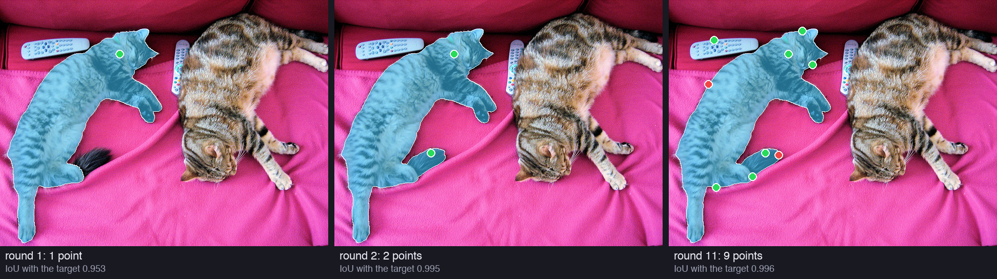
We played the same game with the released model: the target is the left cat, and each round follows the rules above.

plain text

target: the left cat (50,517 pixels). Rounds without a new point: [8, 11]
  round  1: first point (233, 105), foreground                                             points 1  IoU 0.953  predicted 1.005
  round  2: point (188, 298) from the error region (2,391 px), foreground (missed pixel)   points 2  IoU 0.995  predicted 1.015
  round  3: point (77, 164) from the error region (253 px), background (extra pixel)       points 3  IoU 0.995  predicted 1.002
  ...
  round  8: no new point: only the previous mask                                           points 7  IoU 0.996  predicted 1.001
  ...
  round 11: no new point: only the previous mask                                           points 9  IoU 0.996  predicted 1.002
noisy box for training: sides 312 x 419 px -> noise std 20.0, 20.0 px (10% of the side, at most 20); box [5, 53, 317, 472] -> [1, 13, 312, 455]; IoU with the target 0.995

Three copies of the photo with the left cat masked in blue. Round 1 has one green point on the cat's head, IoU 0.953. Round 2 adds a green point on the tail, IoU 0.995. Round 11 shows nine points, green and red, IoU 0.996 — Rounds 1, 2 and 11 of the training game. Green points are foreground points (missed pixels), red points are background points (extra pixels). One correction point lifts the IoU from 0.953 to 0.995.

The first random click gives an IoU of 0.953. The first mask missed the tail: the error region has 2,391 pixels, and the second point lands on the tail. After it, the IoU is 0.995 and the error region shrinks to about 250 pixels at the edge. The later rounds change little. Our target is SAM's own mask, so the released model starts close to it. During training, with real annotated masks and a model that is still learning, the errors are much larger.

Look also at the column "predicted". The IoU head says 1.005 and 1.015. A true IoU can never be above 1. The IoU head is a plain MLP with no limit at the end, so it can overshoot a little when it is very sure.

The training recipe completes the appendix:

From the paper§Apage 17

What it says

"AdamW", a "warmup for 250 iterations", a learning rate of "8e−4", "90k iterations (∼2 SA-1B epochs)", decreases by 10 at 60k and at 86,666 iterations, "The batch size is 256 images", "weight decay (wd) to 0.1", "drop path (dp) with a rate of 0.4", "layer-wise learning rate decay (ld) of 0.8", "No data augmentation is applied", "256 GPUs", and "up to 64 randomly sampled masks per GPU". Masks that "cover more than 90% of the image" are removed.

What it means

AdamW is the standard rule that turns gradients into weight updates. An epoch is one full pass over the dataset, and a batch is the set of pictures of one update.

90,000 iterations of 256 pictures is 23 million pictures, about two passes over SA-1B. That is a short training for a model of this size, because each picture carries about 100 masks. With up to 64 masks per picture and 11 rounds each, the decoder runs up to 704 times for each encoder pass. The game of clicks is cheap only because of the split into a heavy encoder and a light decoder.

"No data augmentation" is a confident choice. Most vision models flip, crop and recolour their training pictures to see more variety. SA-1B is so large and so varied that SAM does not need it. The masks that cover almost the whole picture are removed, because "the whole picture" is rarely the object that a user wants.

Our script did the arithmetic and drew the schedule:

plain text

90,000 iterations x 256 images = 23,040,000 pictures seen = 2.09 passes over 11M pictures
masks: up to 64 per GPU, 1 picture per GPU (256 pictures on 256 GPUs) -> up to 704 decoder runs per picture per iteration (64 masks x 11 rounds)

The learning rate of SAM training. It rises to 0.0008 in the first 250 iterations, stays there until iteration 60,000, drops to 0.00008, and drops again to 0.000008 at iteration 86,666, until the end at 90,000.

The layer-wise decay gives each block of the encoder its own learning rate. The paper gives only the factor 0.8. With the usual rule of the MAE code, each block gets 0.8 times the rate of the block above it:

plain text

  mask decoder and neck  8e-4 x 0.8^0  = 8.00e-04
  block 32 (last)        8e-4 x 0.8^1  = 6.40e-04
  block 16               8e-4 x 0.8^17 = 1.80e-05
  block 1 (first)        8e-4 x 0.8^32 = 6.34e-07
  patch embedding        8e-4 x 0.8^33 = 5.07e-07

The first block learns about 1,260 times more slowly than the decoder. MAE already taught the early blocks to see edges and textures, and SAM keeps that knowledge almost unchanged. The late blocks and the new decoder do most of the learning.

Key takeaways

Three blocks, two budgets. The image encoder (637 million weights, 5.96 TFLOPs) runs once for each picture. The prompt encoder (6,476 weights) and the mask decoder (4.06 million weights) run for each click and need 0.06% of the encoder's work.
The encoder is a ViT-H/16 with windows. 4,096 tokens of 1,280 numbers pass through 32 blocks. 28 blocks attend inside 25 windows of 14 × 14 tokens (17.5 times fewer attention scores); blocks 8, 16, 24 and 32 attend globally. A neck shrinks the output to 256 × 64 × 64.
A click is "where" plus "what kind". The position becomes 256 random Fourier features (128 sines, 128 cosines, length 11.31), and a learned type vector is added. A box is two such tokens; a mask is added to the image grid.
The decoder is two-way. Two layers of four steps: tokens talk, tokens read the image, an MLP, and the image reads the tokens. Our hand-written version matches the model's masks to 0.0004.
A mask is a dot product. Each mask token becomes 32 numbers; each pixel of the 256 × 256 upscaled grid has 32 numbers. At the cat's body, the ear token gives −22.51 and the cat token gives +4.14.
Ambiguity is solved by "best of three". Three mask tokens give three masks, and only the one with the lowest loss learns. A fourth token serves the clear case of several prompts. A single averaged output would be 88 times worse for the ear.
The loss: 20 × focal + dice for the best mask, plus the squared error of the IoU head. For the ear click, the minimum is mask 2 (0.0152) for the target "ear". It is mask 3 (0.0471) for the target "cat".
Training is a game of 11 clicks per mask, with corrections from the error region and two rounds of self-refinement. It is affordable only because the decoder is so light.

Next, in Part 4: the data engine and SA-1B. How the three stages of annotation worked, how SAM made 1.1 billion masks by itself, and how the team checked their quality.

Run it yourself

The script code/papers/sam/sam_part3.py reads the configuration and counts the weights of the three models. It follows the shapes through ViT-H and computes the positional code of the click by hand. It runs the mask decoder again by hand, counts the FLOPs and times each part. It also computes the losses and plays the 11-round training game. Every number of this part is in results/part3.json.

bash

pip install torch transformers datasets pillow
python sam_part3.py        # uses facebook/sam-vit-base, -large and -huge (about 3.8 GB in total)

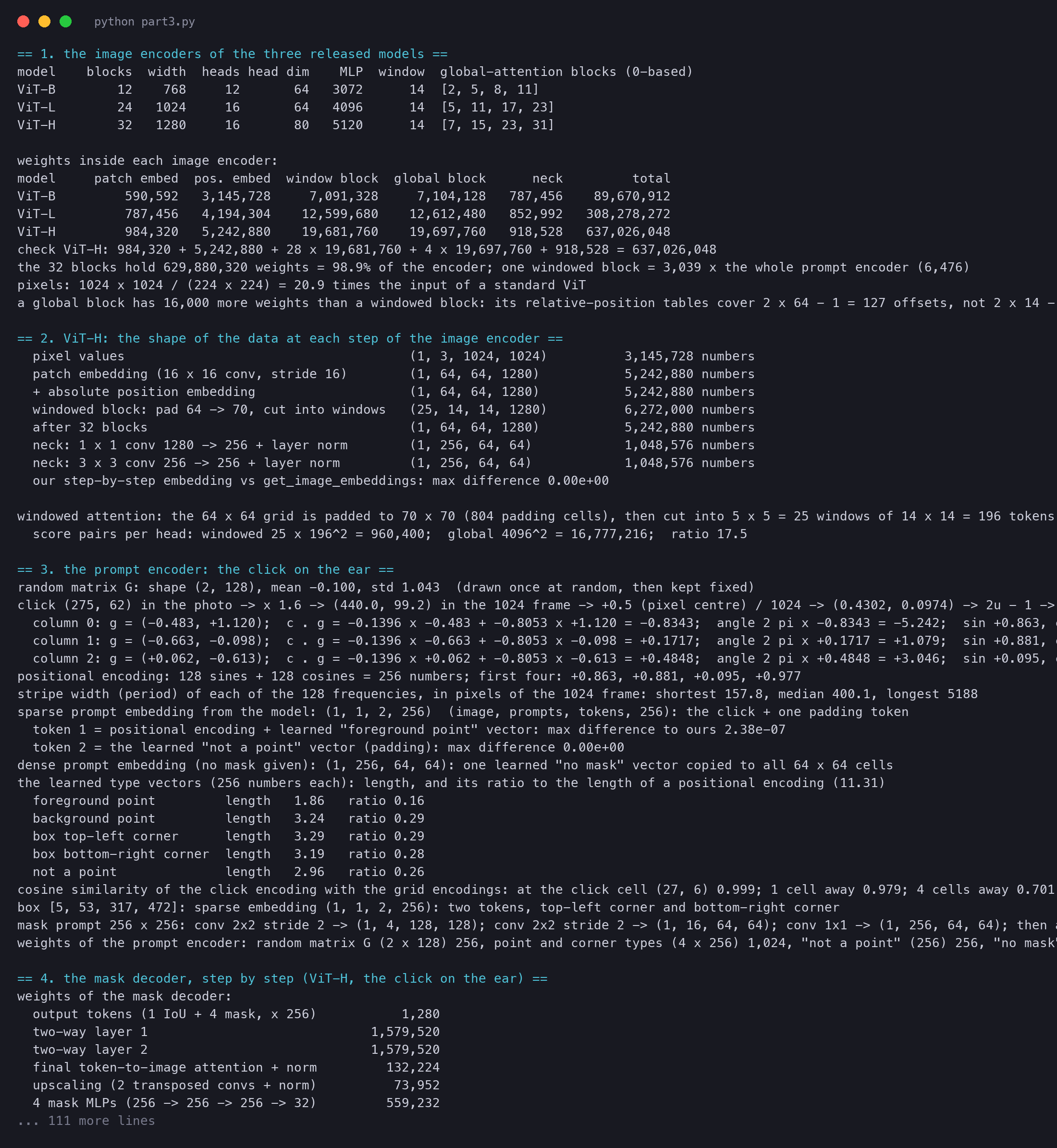
Terminal output of sam_part3.py: the configuration and weights of the three image encoders, the shapes through ViT-H, the windowed attention numbers, and the positional encoding of the click worked by hand — The first part of the output of sam_part3.py, as it ran for this article.

The paper and the code

Segment Anything (ICCV 2023) · code and weights · our scripts for this part

The Model: Encoder, Prompts and Decoder

Figure 4: the model in one picture#

The image encoder#

Attention, the step that mixes the tokens#

Windowed and global attention#

The prompt encoder#

The positional encoding of a click#

Masks as prompts#

The mask decoder#

From tokens to a mask#

Resolving ambiguity#

Efficiency#

The losses#

Focal loss: grade the hard pixels#

Dice loss: grade the overlap#

The IoU head: grade the grader#

All together: the minimum over three masks#

Training: a game of clicks#

The paper and the code#

Figure 4: the model in one picture

The image encoder

Attention, the step that mixes the tokens

Windowed and global attention

The prompt encoder

The positional encoding of a click

Masks as prompts

The mask decoder

From tokens to a mask

Resolving ambiguity

Efficiency

The losses

Focal loss: grade the hard pixels

Dice loss: grade the overlap

The IoU head: grade the grader

All together: the minimum over three masks

Training: a game of clicks

The paper and the code