BERT, explained · Background · Covers From n-grams (1948) to UltraBERT (2026)
Before and After BERT
How machines learned to read: from counting word pairs to word vectors, recurrent networks, attention and pre-training, then BERT and everything after it, up to 2026. With the maths of each step and small runs you can check.
BERT: Pre-training of Deep Bidirectional Transformers for Language Understanding. Jacob Devlin, Ming-Wei Chang, Kenton Lee, Kristina Toutanova. NAACL 2019, 2018. arXiv:1810.04805
BERT did not come from nowhere. It joined three ideas that took decades to grow: words as vectors, attention, and pre-training on plain text. After BERT, the field split into new branches. One of them grew into the chat models of today, and BERT's own branch is still growing in 2026.
This page tells that story in order, with the key equation of each step and a small run you can check. Read it before Part 1 if you want the background, or after Part 6 to see where BERT stands.
The road to BERT and beyond. Blue steps came before BERT; orange steps came after it. Each step fixed a weakness of the one before.
Every model on this page answers the same question in some form: given some words, which word fits here? A model that answers it well has learned a lot about language. To guess the word after "The capital of France is", it must know some geography. To guess the word after "She dropped the glass and it", it must know some physics.
The question can be asked in two ways, and the difference matters for BERT. A left-to-right model sees only the words before the gap and guesses the next word. A fill-in-the-blank model sees the words on both sides of the gap. BERT is the second kind. Most of the models before it, and most of the famous ones after it, are the first kind.
The oldest method is to count. In 1948, the mathematician Shannon showed how to imitate English text. He picked each letter or word from counts of what followed the previous ones. This became the n-gram model, the standard tool of speech recognition and translation for decades.
The idea is simple. To guess the word after "the", look at every "the" in a large text and count the words that follow it. If "first" follows "the" 1.2% of the time, then the model says P(first∣the)=0.012.
P(wt∣wt−1)=count(wt−1)count(wt−1,wt)
Read it this way. The left side, P(wt∣wt−1), is the probability of word wt given the word just before it. The top of the fraction counts how often the pair appears. The bottom counts how often the first word appears at all. This is a bigram model: it looks back one word. A trigram looks back two words, and an n-gram looks back n−1.
A tiny example. Suppose the text is "the cat sat. the cat ran. the dog sat." The word "the" appears 3 times. It is followed by "cat" twice and by "dog" once. So P(cat∣the)=2/3 and P(dog∣the)=1/3.
We measure how good a language model is with perplexity:
perplexity=exp(−N1t=1∑NlogP(wt∣wt−1))
The sum adds the log probability that the model gave each real word of a test text, and N is the number of words. A perplexity of 100 means that the model is, on average, as unsure as if it had to choose among 100 equally likely words. Lower is better.
We built a bigram model of WikiText-2, a collection of Wikipedia articles of about 1.7 million words. We counted on the training part and scored on the test part. A pair never seen in training would get probability 0 and an infinite perplexity, so a model needs smoothing. We tried two kinds:
python
def p_bigram(prev, w): """Add-one smoothing: every pair gets one extra imaginary count, so no probability is zero.""" return (bi[(prev, w)] + 1) / (uni[prev] + V)def p_interp(prev, w, lam=0.7): """Interpolation: trust the pair count with weight lam, fall back on the single-word count otherwise.""" ml = bi[(prev, w)] / uni[prev] if uni[prev] else 0.0 return lam * ml + (1 - lam) * p_unigram(w)
plain text
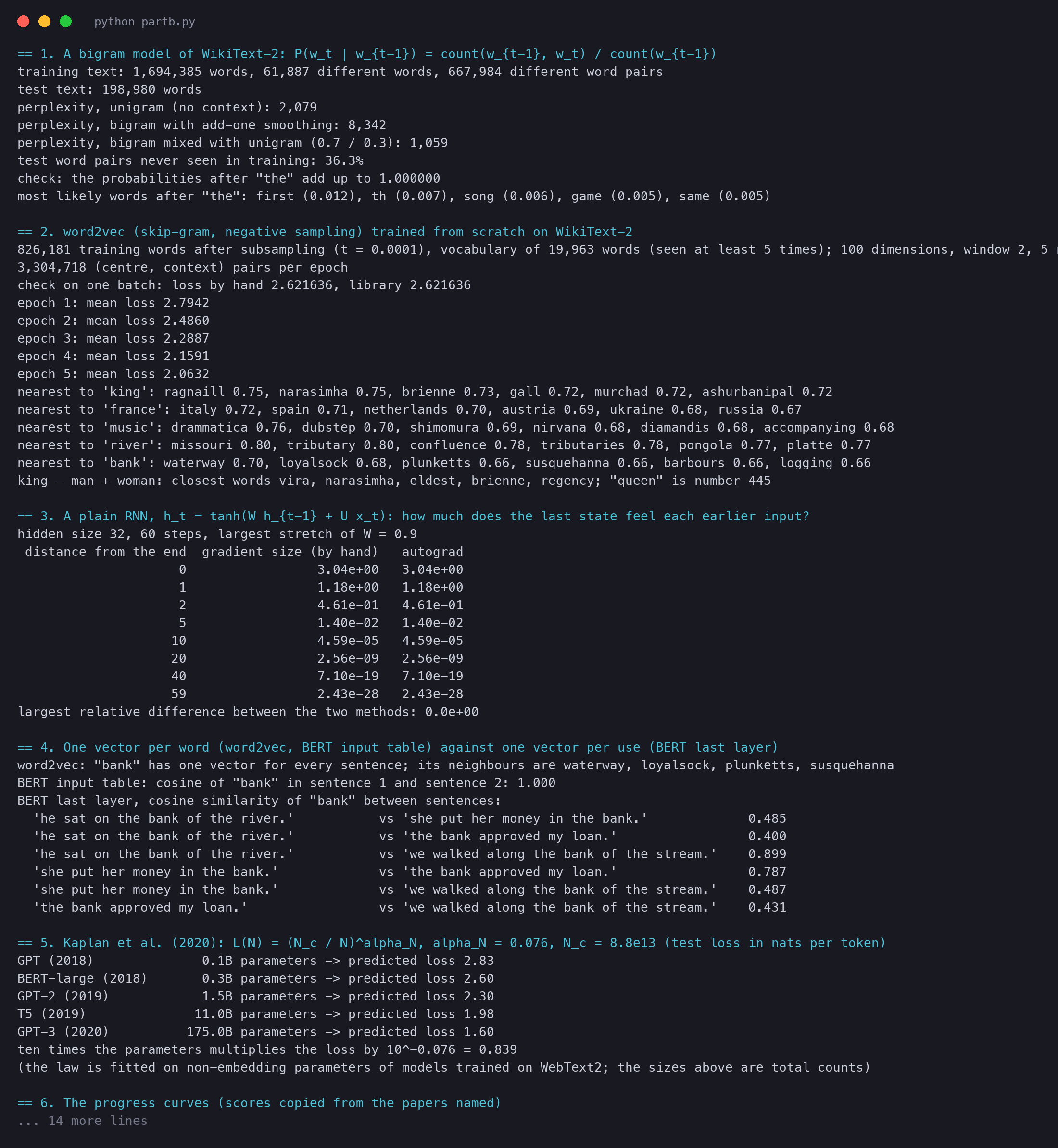
== 1. A bigram model of WikiText-2: P(w_t | w_{t-1}) = count(w_{t-1}, w_t) / count(w_{t-1})training text: 1,694,385 words, 61,887 different words, 667,984 different word pairstest text: 198,980 wordsperplexity, unigram (no context): 2,079perplexity, bigram with add-one smoothing: 8,342perplexity, bigram mixed with unigram (0.7 / 0.3): 1,059test word pairs never seen in training: 36.3%check: the probabilities after "the" add up to 1.000000
Our run on WikiText-2. One word of context halves the perplexity, but only with good smoothing. Add-one smoothing gives too much probability to pairs that never occur, and does worse than no context at all.
The result shows both the power and the weakness of counting. With one word of context and good smoothing, the perplexity falls from 2,079 to 1,059. With naive smoothing it gets worse, 8,342, because add-one gives too much probability to the 61,887 words that could follow each word.
The deeper problem is the last useful line: 36.3% of the word pairs in the test text never appear in the 1.7 million training words. Counting cannot generalise. The pair "cat sat" teaches it nothing about "dog sat", because to a counter, "cat" and "dog" are just different symbols. Longer contexts make this worse, since most triples and quadruples are never seen at all.
The fix is to give each word a list of numbers, a vector, so that similar words get similar vectors. Then "dog sat" can borrow from "cat sat", because "dog" and "cat" are close. Yoshua Bengio and colleagues showed in 2003 that a neural network can learn such vectors while it learns to predict the next word. It worked, but it was slow.
The second word2vec paper gave the training objective that most people use, skip-gram with negative sampling. The skip-gram idea: for each word in the text, predict the words around it.
Here is the objective for one centre word wI and one real neighbour wO, written as a loss to make small:
L=−logσ(uwO⊤vwI)−i=1∑klogσ(−uwi⊤vwI)
Read it this way. vwI is the vector of the centre word, and uwO is the vector of the real neighbour. Each word has two vectors: one for when it is the centre, one for when it is a neighbour. The dot product u⊤v is large when the two vectors point the same way. The sigmoid σ(z)=1/(1+e−z) turns it into a number between 0 and 1. The words w1,…,wk are k random noise words.
A tiny example. If the real pair has dot product 2, then σ(2)=0.88 and −log0.88=0.13, a small loss. If one noise word also has dot product 2, its term is −logσ(−2)=−log0.12=2.13, a large loss. Training pushes the real pair together and the noise pair apart.
We trained skip-gram with negative sampling from scratch on WikiText-2 in PyTorch. Method 1 is the loss written as above. Method 2 asks PyTorch's binary cross-entropy the same yes-or-no question. Both must agree:
python
def sgns_loss_by_hand(c, o, k): """Method 1, the paper's objective: -log s(u_o . v_c) - sum over k noise words of log s(-u_k . v_c).""" vc = v_in(c) # (B, DIM) pos = (u_out(o) * vc).sum(-1) # (B,) score of the real context word neg = torch.bmm(u_out(k), vc[:, :, None])[..., 0] # (B, K) scores of the noise words return -(F.logsigmoid(pos) + F.logsigmoid(-neg).sum(-1)).mean()def sgns_loss_library(c, o, k): """Method 2: the same as binary classification, real pair = 1, noise pair = 0, with PyTorch's BCE.""" vc = v_in(c) logits = torch.cat([(u_out(o) * vc).sum(-1, keepdim=True), torch.bmm(u_out(k), vc[:, :, None])[..., 0]], 1) labels = torch.cat([torch.ones_like(logits[:, :1]), torch.zeros_like(logits[:, 1:])], 1) return F.binary_cross_entropy_with_logits(logits, labels, reduction='none').sum(-1).mean()
plain text
== 2. word2vec (skip-gram, negative sampling) trained from scratch on WikiText-2826,181 training words after subsampling (t = 0.0001), vocabulary of 19,963 words (seen at least 5 times); 100 dimensions, window 2, 5 negatives, 5 epochs3,304,718 (centre, context) pairs per epochcheck on one batch: loss by hand 2.621636, library 2.621636epoch 1: mean loss 2.7942epoch 5: mean loss 2.0632nearest to 'king': ragnaill 0.75, narasimha 0.75, brienne 0.73, gall 0.72, murchad 0.72, ashurbanipal 0.72nearest to 'france': italy 0.72, spain 0.71, netherlands 0.70, austria 0.69, ukraine 0.68, russia 0.67nearest to 'river': missouri 0.80, tributary 0.80, confluence 0.78, tributaries 0.78, pongola 0.77, platte 0.77nearest to 'bank': waterway 0.70, loyalsock 0.68, plunketts 0.66, susquehanna 0.66, barbours 0.66, logging 0.66king - man + woman: closest words vira, narasimha, eldest, brienne, regency; "queen" is number 445
The two losses agree to six decimal places. The neighbours show what word vectors learn. "France" sits among other European countries, and "river" among tributaries and confluences. "King" sits among the names of kings from the Wikipedia articles, which is not wrong: the model groups words that occur in the same places.
The famous analogy fails here: "queen" comes 445th. Our text is under 2 million words; the paper's Google News text had 6 billion. Vector arithmetic needs a lot of reading before the directions line up. Keep this in mind, because it is exactly why pre-training on huge text became the rule.
Now look at "bank". Its neighbours are all about rivers: waterway, Susquehanna, Loyalsock Creek. In these Wikipedia articles, banks are mostly river banks. A money bank in a new sentence would get the same vector, because word2vec has one vector per word. That is the limit that ELMo and BERT remove.
Word vectors give each word a meaning, but a sentence is more than a bag of words. "Dog bites man" and "man bites dog" use the same words. A recurrent neural network, or RNN, reads the words in order and keeps a running summary, its hidden state:
ht=tanh(Wht−1+Uxt)
Read it this way. xt is the vector of word t. ht−1 is the summary of everything before it. The matrices W and U mix the old summary with the new word, and tanh squeezes each number into the range −1 to 1. The new summary ht is passed on to the next word. One network, used again at every step, can read a sentence of any length.
The trouble is training. To learn that the first word matters for the last, the error signal must travel back through every step. At each step it is multiplied by W and by the slope of tanh. If those multiply to less than 1, the signal shrinks at every step and soon vanishes. This is the vanishing gradient problem.
A tiny example. If each step multiplies the signal by 0.5, then after 10 steps it is 0.510≈0.001 of its size. After 20 steps it is about one millionth.
We measured it. We built a plain RNN with 32 numbers in its hidden state and ran it over 60 random inputs. We then asked how much the last state changes when each input changes. Method 1 walks back step by step and multiplies the slopes by hand. Method 2 asks PyTorch's autograd:
python
# Method 1: walk back through the steps. d loss / d h_t = J_{t+1}^T ... J_T^T target, with J_t = diag(1 - h_t^2) Wg, by_hand = target.clone(), [None] * Tfor t in range(T - 1, -1, -1): pre = (1 - hs[t] ** 2) * g # through the tanh of step t by_hand[t] = (Uin.T @ pre).norm().item() # gradient that reaches input x_t g = W.T @ pre # pass on to h_{t-1}# Method 2: autogradloss.backward()auto = xs.grad.norm(dim=1).tolist()
plain text
== 3. A plain RNN, h_t = tanh(W h_{t-1} + U x_t): how much does the last state feel each earlier input?hidden size 32, 60 steps, largest stretch of W = 0.9 distance from the end gradient size (by hand) autograd 0 3.04e+00 3.04e+00 1 1.18e+00 1.18e+00 2 4.61e-01 4.61e-01 5 1.40e-02 1.40e-02 10 4.59e-05 4.59e-05 20 2.56e-09 2.56e-09 40 7.10e-19 7.10e-19 59 2.43e-28 2.43e-28largest relative difference between the two methods: 0.0e+00
Our run. The signal that reaches each earlier word falls by a nearly constant factor per step. Ten words back it is 66,000 times weaker than at the last word; fifty-nine words back it is gone.
Both methods agree exactly. Ten words back, the signal is 66,000 times weaker than at the last word. Twenty words back it is a billion times weaker. A plain RNN cannot learn that a word at the start of a paragraph matters for a word at the end.
The LSTM (long short-term memory), published by Hochreiter and Schmidhuber in 1997, fixed much of this. It adds a separate memory cell and gates that decide what to keep, what to forget and what to output. Because the cell is updated by addition rather than repeated multiplication, a signal can pass through many steps without fading. By 2014, LSTMs were the standard tool for text.
A tiny example. Three input words have scores 2, 0 and 0 for the current output word. Then e2=7.39 and e0=1, so the weights are 7.39/9.39=0.79, then 0.11 and 0.11. The context vector is 79% the first word's state. Change the output word, and the scores and weights change with it.
By 2017, every good translation model was an RNN with attention on top. The RNN still read the words one at a time, so training could not use the full parallel power of a GPU.
Attention(Q,K,V)=softmax(dkQK⊤)V
This is Bahdanau's weighted sum again, done for all words at once with matrices. Q, K and V hold the queries, keys and values of all words as rows, and dk is the length of a key. Dividing by dk keeps the scores in a range where the softmax still learns. The Transformer series works through it in full; here we need only the idea that every word reads every other word in one step.
The Transformer had two halves, an encoder and a decoder, for translation. The next year, two groups took one half each. GPT took the decoder. BERT took the encoder.
All the models so far were trained for one task at a time, from scratch or from word vectors. In 2018, three papers showed a better way: train a language model on lots of plain text first, then reuse it.
ELMoktask=γtaskj=0∑Lsjtaskhk,jLM
Read it this way. k is the position of the token. hk,jLM is the state of token k in layer j of the two-way language model; layer 0 is the plain word vector. The weights sj come from a softmax, so they add up to 1. γ scales the whole vector. With two LSTM layers, L=2, and a task might learn weights such as 0.2, 0.3 and 0.5 for layers 0, 1 and 2.
GPT's fine-tuning loss adds the language model loss as a helper, with a weight λ:
L3(C)=L2(C)+λ⋅L1(C)
L2 is the loss of the task, for example the log probability of the right label. L1 is the next-word loss on the same task text. Keeping a little of the old job while learning the new one helps the model not to forget what it learned in pre-training.
To compare all these models, the field needed one test. It arrived in the same year.
In October 2018, BERT joined the pieces. From word2vec it took the idea that vectors learned from plain text carry meaning. From ELMo it took vectors that depend on the whole sentence. From GPT it took the Transformer and pre-training with fine-tuning. Its own new step was to train a Transformer encoder that sees both sides of every word at once, in every layer.
A left-to-right model cannot simply look right too: each word would then see the very word it must predict. BERT's fix is the masked language model. It hides 15% of the tokens and asks the model to fill them in:
LMLM=−i∈M∑logP(xi∣x∖M)
Read it this way. M is the set of masked positions. x∖M is the sentence with those positions hidden. For each hidden position i, the model gives a probability to the real token xi, using every visible token on both sides. The loss is the sum of the negative log probabilities. Part 3 works through it on the real model, including the 80/10/10 rule for what replaces a masked token.
The result was a jump. On the GLUE leaderboard, GPT had a score of 72.8. BERT-large reached 80.5, a gain of 7.7 points in four months.
Does BERT really give each use of a word its own vector? We ran the released BERT-base on four sentences with "bank". In the input table, "bank" has one vector, as in word2vec. After the twelve layers, each "bank" has its own:
plain text
== 4. One vector per word (word2vec, BERT input table) against one vector per use (BERT last layer)word2vec: "bank" has one vector for every sentence; its neighbours are waterway, loyalsock, plunketts, susquehannaBERT input table: cosine of "bank" in sentence 1 and sentence 2: 1.000BERT last layer, cosine similarity of "bank" between sentences: 'he sat on the bank of the river.' vs 'she put her money in the bank.' 0.485 'he sat on the bank of the river.' vs 'the bank approved my loan.' 0.400 'he sat on the bank of the river.' vs 'we walked along the bank of the stream.' 0.899 'she put her money in the bank.' vs 'the bank approved my loan.' 0.787 'she put her money in the bank.' vs 'we walked along the bank of the stream.' 0.487 'the bank approved my loan.' vs 'we walked along the bank of the stream.' 0.431
Our run with BERT-base. The two river banks are close (0.899) and the two money banks are close (0.787). Across the two meanings the similarity drops to 0.40 to 0.49.
The river bank and the stream bank have a similarity of 0.899, though the sentences share almost no other words. The two money banks have 0.787. Across the two meanings, the similarity falls to between 0.400 and 0.487. BERT sorted the four uses by meaning without being told that "bank" has two meanings. That is the problem of Step 2, solved.
Parts 1 to 6 read the BERT paper itself, line by line. The rest of this page jumps ahead to what happened next.
The learning curve of the field. GLUE (top) climbed from 70.0 to 90.3 in eighteen months and passed its human baseline in 2019. Its harder successor, SuperGLUE (bottom), climbed from BERT's 69.0 to 89.9 in under two years.
The curve has one shape twice. Each benchmark starts with a large gap below the human line, closes it in a year or two, and then has little room left. On GLUE, BERT closed more than half of the gap between GPT and the human baseline in one step. SuperGLUE was designed to be hard for BERT. Even so, models went from 69.0 to above its human level of 89.8 in less than two years. The dates are those of the papers or the leaderboard entries they report.
Two cautions. First, "human performance" here is the score of paid crowd workers with short training, not of experts. Second, passing the human line on a benchmark does not mean that a model understands language as people do. It means that the benchmark has stopped telling good models apart.
After BERT, work split into three branches, following the three ways to use a Transformer.
Encoders, like BERT. They read the whole input at once and are best at understanding: classification, search, finding names in text. RoBERTa, ALBERT, ELECTRA and DeBERTa refine this branch. Part 6 covers each of them.
Encoder-decoders, like the original Transformer. They read an input and write an output. T5 and BART belong here.
Decoders, like GPT. They read left to right and write the next token. GPT-2 and GPT-3 grew this branch, and today's chat models come from it.
The size curve. On a log scale, each step up the grid is ten times more parameters. From GPT in 2018 to GPT-3 in 2020, the largest models grew 1,750 times.L(N)=(NNc)αN
Read it this way. N is the number of parameters, not counting the word vector tables. L is the test loss in nats per token, the average negative log probability of the next token. Nc and αN are two constants fitted to the authors' measurements.
A tiny example. Make a model 10 times bigger. The new loss is (Nc/10N)0.076=L(N)×10−0.076=0.839L(N). So each tenfold step cuts the loss by about 16%, whatever the starting size. We applied the law at the sizes the GPT-3 paper lists:
plain text
== 5. Kaplan et al. (2020): L(N) = (N_c / N)^alpha_N, alpha_N = 0.076, N_c = 8.8e13 (test loss in nats per token)GPT (2018) 0.1B parameters -> predicted loss 2.83BERT-large (2018) 0.3B parameters -> predicted loss 2.60GPT-2 (2019) 1.5B parameters -> predicted loss 2.30T5 (2019) 11.0B parameters -> predicted loss 1.98GPT-3 (2020) 175.0B parameters -> predicted loss 1.60ten times the parameters multiplies the loss by 10^-0.076 = 0.839(the law is fitted on non-embedding parameters of models trained on WebText2; the sizes above are total counts)
These are predictions for left-to-right models on the authors' web text, not measured losses of BERT or T5, which were trained differently. The point is the shape: from GPT to GPT-3, the law predicts the loss falls from 2.83 to 1.60. Because the gains were predictable, companies could plan and pay for very large training runs. That is how the decoder branch grew so fast.
If decoders can do everything, why does anyone still train encoders? Because for many jobs, an encoder is far cheaper. Think of deciding whether an email is spam, or finding the ten documents closest to a question. You need a good vector for the text, not a written answer. An encoder gives that vector in one pass.
ModernBERT is not a new idea. It is BERT rebuilt with six years of lessons from the decoder world. Think of a classic car with a new engine, new brakes and new tyres. The body is the same, and it does the same job, but faster. Here is what changed, read from the two released models.
python
for k, n in NAMES.items():
    c = AutoConfig.from_pretrained(n)
    rows[k] = dict(layers=c.num_hidden_layers, hidden=c.hidden_size, ffn=c.intermediate_size,
                   heads=c.num_attention_heads, vocab=c.vocab_size, max_len=c.max_position_embeddings,
                   params=sum(p.numel() for p in mlm[k].parameters()) / 1e6)
plain text
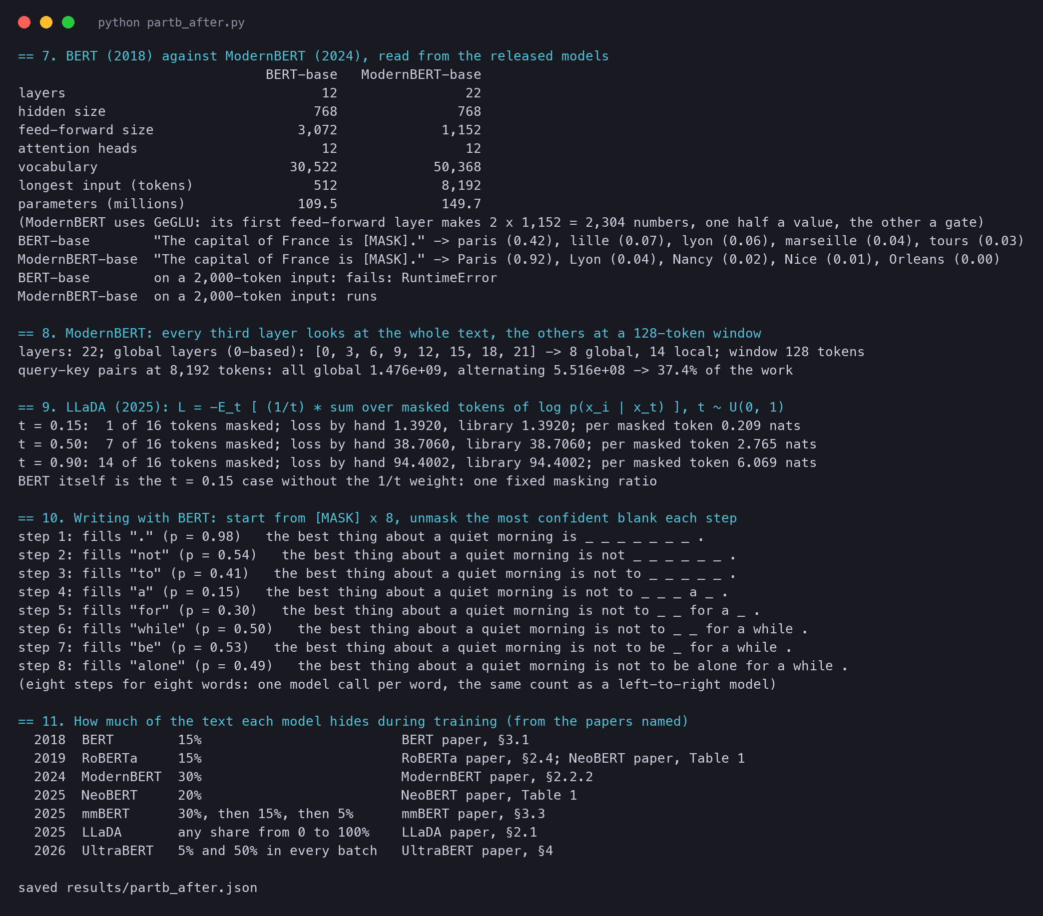
== 7. BERT (2018) against ModernBERT (2024), read from the released models BERT-base ModernBERT-baselayers 12 22hidden size 768 768feed-forward size 3,072 1,152attention heads 12 12vocabulary 30,522 50,368longest input (tokens) 512 8,192parameters (millions) 109.5 149.7(ModernBERT uses GeGLU: its first feed-forward layer makes 2 x 1,152 = 2,304 numbers, one half a value, the other a gate)
The width is the same, 768 numbers per token, but ModernBERT is almost twice as deep: 22 layers against 12. The paper calls this "Deep & Narrow" and chose it because deeper models did better on tasks at the same size. The vocabulary grew from 30,522 to 50,368 pieces, because the new tokenizer also has to cut up code. The longest input grew sixteen times, from 512 to 8,192 tokens.
Two of the changes come straight from decoders. RoPE replaces BERT's table of learned position vectors, so the model is not tied to the positions it saw in training. GeGLU replaces the plain feed-forward layer. One half of its numbers is a value, and the other half is a gate that decides how much of each value passes.
plain text
== 8. ModernBERT: every third layer looks at the whole text, the others at a 128-token windowlayers: 22; global layers (0-based): [0, 3, 6, 9, 12, 15, 18, 21] -> 8 global, 14 local; window 128 tokensquery-key pairs at 8,192 tokens: all global 1.476e+09, alternating 5.516e+08 -> 37.4% of the work
Eight of the 22 layers are global. At the full length, the attention does 37.4% of the work that 22 global layers would do. That count leaves out the feed-forward layers, so it is a share of the attention cost only. ModernBERT also drops padding tokens before the first layer ("unpadding"), so a batch of short and long texts wastes no work on empty places.
Does all this change what the model knows? Here is the same blank for both models:
plain text
BERT-base "The capital of France is [MASK]." -> paris (0.42), lille (0.07), lyon (0.06), marseille (0.04), tours (0.03)ModernBERT-base "The capital of France is [MASK]." -> Paris (0.92), Lyon (0.04), Nancy (0.02), Nice (0.01), Orleans (0.00)BERT-base on a 2,000-token input: fails: RuntimeErrorModernBERT-base on a 2,000-token input: runs
Both models know the answer, but ModernBERT is far surer: 0.92 against 0.42. It also keeps capital letters (BERT-base lower-cases everything). And it reads a 2,000-token text in one pass, where BERT stops with an error, because it has no position vector after place 512.
ModernBERT started a small revival. In the next two years, groups built new encoders, tested encoders against decoders fairly, and found a way to make BERT's own objective write text. One question ran through all of it: how much of the text should the model hide?
BERT can fill blanks, but it cannot write a paragraph. Or can it? Start with a row of blanks, fill the one you are surest about, and repeat. Image models such as Stable Diffusion work in a similar way: they start from noise and remove a little of it at each step. For text, the "noise" is the [MASK] token.
We computed the loss two ways on BERT's own predictions, once by hand and once with PyTorch's cross-entropy, at three masking levels:
python
    m = inner[torch.rand(len(inner), generator=g) < t]     # forward process: each token masked with probability t
    xt = x0.clone()
    xt[m] = tok[k].mask_token_id
    with torch.no_grad():
        logits = mlm[k](input_ids=xt[None]).logits[0].double()   # float64, so the two methods can agree closely
    # Method 1: by hand. log-softmax of the true token at every masked place, summed, times 1/t
    logp = logits[m] - logits[m].logsumexp(-1, keepdim=True)
    hand = -(1 / t) * logp.gather(1, x0[m][:, None]).sum()
    # Method 2: the library. cross-entropy summed over masked places, then the same 1/t weight
    lib = (1 / t) * F.cross_entropy(logits[m], x0[m], reduction='sum')
plain text
== 9. LLaDA (2025): L = -E_t [ (1/t) * sum over masked tokens of log p(x_i | x_t) ], t ~ U(0, 1)t = 0.15: 1 of 16 tokens masked; loss by hand 1.3920, library 1.3920; per masked token 0.209 natst = 0.50: 7 of 16 tokens masked; loss by hand 38.7060, library 38.7060; per masked token 2.765 natst = 0.90: 14 of 16 tokens masked; loss by hand 94.4002, library 94.4002; per masked token 6.069 natsBERT itself is the t = 0.15 case without the 1/t weight: one fixed masking ratio
The two methods agree. Look at the loss per hidden token: 0.209 when BERT sees most of the sentence, 6.069 when almost all of it is hidden. BERT was trained only at 15%, so it never practised with a nearly empty sentence. A writing model must start from an empty one, and that is why LLaDA trains at every masking level.
So can plain BERT write, with no extra training? We gave bert-base-uncased a prompt and eight blanks. At each step, it fills the one blank it is surest about:
Writing with BERT, one blank per step (our run, bert-base-uncased, no extra training). The teal token is the one filled at that step, orange boxes are still blank, and p is BERT's probability for the new token.
plain text
== 10. Writing with BERT: start from [MASK] x 8, unmask the most confident blank each stepstep 1: fills "." (p = 0.98) the best thing about a quiet morning is _ _ _ _ _ _ _ .step 2: fills "not" (p = 0.54) the best thing about a quiet morning is not _ _ _ _ _ _ .step 3: fills "to" (p = 0.41) the best thing about a quiet morning is not to _ _ _ _ _ .step 4: fills "a" (p = 0.15) the best thing about a quiet morning is not to _ _ _ a _ .step 5: fills "for" (p = 0.30) the best thing about a quiet morning is not to _ _ for a _ .step 6: fills "while" (p = 0.50) the best thing about a quiet morning is not to _ _ for a while .step 7: fills "be" (p = 0.53) the best thing about a quiet morning is not to be _ for a while .step 8: fills "alone" (p = 0.49) the best thing about a quiet morning is not to be alone for a while .
BERT writes a correct sentence: "the best thing about a quiet morning is not to be alone for a while".
Look at the order. It fills the full stop first, at 0.98, because it is sure the sentence ends there. Then it writes from both ends: "a" near the end comes before "be" in the middle. A left-to-right model cannot do this. The weak point is also visible: "a" got only 0.15, a guess made with almost nothing around it. Training at every masking level, as LLaDA does, is what makes those early steps reliable.
The masking ratio started as one number in the BERT paper. Eight years later, it is the main design choice of the encoder branch:
How much of the text each model hides during training, from the papers named. BERT and RoBERTa used 15%; ModernBERT doubled it; mmBERT lowers it stage by stage; LLaDA draws a new share for every sequence; UltraBERT uses 5% and 50% together.
Each row fixed the weakness in the row above. That is the "curve of learning" of the whole field: not one leap, but a chain of fixes, each one possible only because of the last.
Our runs used small data and small models on a laptop. The bigram model and our word2vec saw 1.7 million words of Wikipedia; the real systems saw billions, and our analogy test failed for that reason. Our RNN had random weights and was never trained; it shows how the signal fades, not how a trained LSTM behaves. The scaling numbers are the law's predictions, not measured losses. The benchmark scores are copied from the papers, with their tables named above, and we did not rerun any of those systems.
Our writing test used plain BERT, which was never trained to start from an empty sentence; it shows the idea of LLaDA, not its quality. The results of UltraBERT come from a preprint that is still under review.
Next:Part 1 reads the BERT paper itself, starting with its title and abstract.
Run it yourself
The script behind this page is code/papers/bert/bert_partb.py. It builds the bigram model and trains word2vec on WikiText-2. It measures the fading gradient of a plain RNN two ways and compares the vectors of "bank" in word2vec and BERT. It also applies the scaling law and prints the benchmark scores with their sources. Every number is saved in results/partb.json. On an Apple M-series laptop it takes about three minutes.
The second script, bert_partb_after.py, covers ModernBERT and after. It compares BERT and ModernBERT, counts the alternating attention, computes the LLaDA loss two ways and lets BERT write. Its numbers are in results/partb_after.json; it runs in about a minute on the CPU.