# Before and After BERT
Author: Ishwar Jangid
Canonical URL: https://ishwarj.com/papers/bert/background-before-and-after-bert/
Updated: 2026-10-21
Source: https://github.com/ishwar6/ishwar-books/blob/main/content/papers/bert/background-before-and-after-bert.md
BERT did not come from nowhere. It joined three ideas that took decades to grow: words as vectors, attention, and pre-training on plain text. After BERT, the field split into new branches. One of them grew into the chat models of today, and BERT's own branch is still growing in 2026.
This page tells that story in order, with the key equation of each step and a small run you can check. Read it before Part 1 if you want the background, or after Part 6 to see where BERT stands.
The road to BERT and beyond. Blue steps came before BERT; orange steps came after it. Each step fixed a weakness of the one before.
## The one question every model answers
Every model on this page answers the same question in some form: given some words, which word fits here? A model that answers it well has learned a lot about language. To guess the word after "The capital of France is", it must know some geography. To guess the word after "She dropped the glass and it", it must know some physics.
The question can be asked in two ways, and the difference matters for BERT. A **left-to-right** model sees only the words before the gap and guesses the next word. A **fill-in-the-blank** model sees the words on both sides of the gap. BERT is the second kind. Most of the models before it, and most of the famous ones after it, are the first kind.
> [!DEFINITION] Language model
> A model that gives a probability to each possible next word, given the words so far. A good language model gives high probability to the words that really come next.
## Before BERT
### Step 1: counting words (n-grams)
The oldest method is to count. In 1948, the mathematician Shannon showed how to imitate English text. He picked each letter or word from counts of what followed the previous ones. This became the **n-gram model**, the standard tool of speech recognition and translation for decades.
The idea is simple. To guess the word after "the", look at every "the" in a large text and count the words that follow it. If "first" follows "the" 1.2% of the time, then the model says $$P(\text{first} \mid \text{the}) = 0.012$$.
$$
P(w_t \mid w_{t-1}) = \frac{\text{count}(w_{t-1}, w_t)}{\text{count}(w_{t-1})}
$$
Read it this way. The left side, $$P(w_t \mid w_{t-1})$$, is the probability of word $$w_t$$ given the word just before it. The top of the fraction counts how often the pair appears. The bottom counts how often the first word appears at all. This is a **bigram** model: it looks back one word. A trigram looks back two words, and an n-gram looks back $$n - 1$$.
A tiny example. Suppose the text is "the cat sat. the cat ran. the dog sat." The word "the" appears 3 times. It is followed by "cat" twice and by "dog" once. So $$P(\text{cat} \mid \text{the}) = 2/3$$ and $$P(\text{dog} \mid \text{the}) = 1/3$$.
We measure how good a language model is with **perplexity**:
$$
\text{perplexity} = \exp\left(-\frac{1}{N} \sum_{t=1}^{N} \log P(w_t \mid w_{t-1})\right)
$$
The sum adds the log probability that the model gave each real word of a test text, and $$N$$ is the number of words. A perplexity of 100 means that the model is, on average, as unsure as if it had to choose among 100 equally likely words. Lower is better.
> [!DEFINITION] Perplexity
> A score for a language model on a test text. It is the exponential of the average negative log probability of the real words. A model that always gives the real word probability 1/50 has perplexity 50.
We built a bigram model of WikiText-2, a collection of Wikipedia articles of about 1.7 million words. We counted on the training part and scored on the test part. A pair never seen in training would get probability 0 and an infinite perplexity, so a model needs **smoothing**. We tried two kinds:
```python
def p_bigram(prev, w):
"""Add-one smoothing: every pair gets one extra imaginary count, so no probability is zero."""
return (bi[(prev, w)] + 1) / (uni[prev] + V)
def p_interp(prev, w, lam=0.7):
"""Interpolation: trust the pair count with weight lam, fall back on the single-word count otherwise."""
ml = bi[(prev, w)] / uni[prev] if uni[prev] else 0.0
return lam * ml + (1 - lam) * p_unigram(w)
```
```text
== 1. A bigram model of WikiText-2: P(w_t | w_{t-1}) = count(w_{t-1}, w_t) / count(w_{t-1})
training text: 1,694,385 words, 61,887 different words, 667,984 different word pairs
test text: 198,980 words
perplexity, unigram (no context): 2,079
perplexity, bigram with add-one smoothing: 8,342
perplexity, bigram mixed with unigram (0.7 / 0.3): 1,059
test word pairs never seen in training: 36.3%
check: the probabilities after "the" add up to 1.000000
```
Our run on WikiText-2. One word of context halves the perplexity, but only with good smoothing. Add-one smoothing gives too much probability to pairs that never occur, and does worse than no context at all.
The result shows both the power and the weakness of counting. With one word of context and good smoothing, the perplexity falls from 2,079 to 1,059. With naive smoothing it gets worse, 8,342, because add-one gives too much probability to the 61,887 words that could follow each word.
The deeper problem is the last useful line: 36.3% of the word pairs in the test text never appear in the 1.7 million training words. Counting cannot generalise. The pair "cat sat" teaches it nothing about "dog sat", because to a counter, "cat" and "dog" are just different symbols. Longer contexts make this worse, since most triples and quadruples are never seen at all.
### Step 2: words as vectors (word2vec)
The fix is to give each word a list of numbers, a **vector**, so that similar words get similar vectors. Then "dog sat" can borrow from "cat sat", because "dog" and "cat" are close. Yoshua Bengio and colleagues showed in 2003 that a neural network can learn such vectors while it learns to predict the next word. It worked, but it was slow.
> [!DEFINITION] Word vector (embedding)
> A list of numbers, often 100 to 300 of them, that stands for one word. Words used in similar ways get vectors that point in similar directions. "Embedding" means the same thing.
> [!PAPER] Mikolov et al. (2013), Efficient Estimation of Word Representations in Vector Space · Abstract · page 1
> [](/img/papers/bert/pb-w2v-abstract.png)
>
> **What it says:** two new model architectures compute "continuous vector representations of words" from very large data sets. It takes "less than a day" to learn high-quality word vectors from a "1.6 billion words" data set.
>
> **What it means:**
>
> This is the paper that made word vectors cheap. Bengio's model had a large network on top of the vectors. word2vec threw almost all of it away. It kept only the vectors and a dot product between them. The model became so simple that it could read a billion words in a day.
>
> The trade was deliberate. A simpler model learns less per word, but it can read a thousand times more words. That lesson, that more data can beat a cleverer model, comes back again and again in this story.
> [!PAPER] Mikolov et al. (2013), Efficient Estimation of Word Representations in Vector Space · §1.1 · page 2
> [](/img/papers/bert/pb-w2v-king.png)
>
> **What it says:** with "simple algebraic operations" on the word vectors, vector("King") minus vector("Man") plus vector("Woman") "results in a vector that is closest to the vector representation of the word Queen".
>
> **What it means:**
>
> This result made word vectors famous. Directions in the vector space seem to carry meaning. The step from "man" to "woman" is about the same as the step from "king" to "queen". Nobody told the model about gender or royalty; it found these directions by reading text.
>
> The result needs a lot of text, as our run below shows. It also has a hidden limit that BERT later fixes: each word gets exactly one vector.
The second word2vec paper gave the training objective that most people use, **skip-gram with negative sampling**. The skip-gram idea: for each word in the text, predict the words around it.
> [!PAPER] Mikolov et al. (2013), Distributed Representations of Words and Phrases · §2 · page 2
> [](/img/papers/bert/pb-w2v-skipgram.png)
>
> **What it says:** the skip-gram model learns word vectors that are useful for "predicting the surrounding words". It must "maximize the average log probability" of every word within $$c$$ positions of each centre word.
>
> **What it means:**
>
> Take the sentence "the cat sat on the mat" and the centre word "sat". With $$c = 2$$, the model must predict "the", "cat", "on" and "the" from "sat" alone. Words that appear in similar company end up with similar vectors, because the same vectors must predict the same neighbours.
> [!PAPER] Mikolov et al. (2013), Distributed Representations of Words and Phrases · §2.2 · page 3
> [](/img/papers/bert/pb-w2v-neg.png)
>
> **What it says:** "Negative sampling" (NEG) replaces the full probability with a simpler objective (Eq. 4): a log sigmoid for the real pair, plus $$k$$ log sigmoids for random "noise" words.
>
> **What it means:**
>
> Computing a real probability means comparing the centre word with every word of the vocabulary, which is slow. Negative sampling asks an easier question: is this pair real, or did I draw it at random? The model learns to say "yes" to the real neighbour and "no" to a few random words. That is enough to learn good vectors, and it is much faster.
Here is the objective for one centre word $$w_I$$ and one real neighbour $$w_O$$, written as a loss to make small:
$$
\mathcal{L} = -\log \sigma\left(u_{w_O}^\top v_{w_I}\right) - \sum_{i=1}^{k} \log \sigma\left(-u_{w_i}^\top v_{w_I}\right)
$$
Read it this way. $$v_{w_I}$$ is the vector of the centre word, and $$u_{w_O}$$ is the vector of the real neighbour. Each word has two vectors: one for when it is the centre, one for when it is a neighbour. The dot product $$u^\top v$$ is large when the two vectors point the same way. The sigmoid $$\sigma(z) = 1 / (1 + e^{-z})$$ turns it into a number between 0 and 1. The words $$w_1, \ldots, w_k$$ are $$k$$ random noise words.
> [!DEFINITION] Sigmoid
> The function $$\sigma(z) = 1 / (1 + e^{-z})$$. It maps any number to the range 0 to 1: large positive numbers go near 1, large negative numbers near 0, and $$\sigma(0) = 0.5$$.
A tiny example. If the real pair has dot product 2, then $$\sigma(2) = 0.88$$ and $$-\log 0.88 = 0.13$$, a small loss. If one noise word also has dot product 2, its term is $$-\log \sigma(-2) = -\log 0.12 = 2.13$$, a large loss. Training pushes the real pair together and the noise pair apart.
We trained skip-gram with negative sampling from scratch on WikiText-2 in PyTorch. Method 1 is the loss written as above. Method 2 asks PyTorch's binary cross-entropy the same yes-or-no question. Both must agree:
```python
def sgns_loss_by_hand(c, o, k):
"""Method 1, the paper's objective: -log s(u_o . v_c) - sum over k noise words of log s(-u_k . v_c)."""
vc = v_in(c) # (B, DIM)
pos = (u_out(o) * vc).sum(-1) # (B,) score of the real context word
neg = torch.bmm(u_out(k), vc[:, :, None])[..., 0] # (B, K) scores of the noise words
return -(F.logsigmoid(pos) + F.logsigmoid(-neg).sum(-1)).mean()
def sgns_loss_library(c, o, k):
"""Method 2: the same as binary classification, real pair = 1, noise pair = 0, with PyTorch's BCE."""
vc = v_in(c)
logits = torch.cat([(u_out(o) * vc).sum(-1, keepdim=True), torch.bmm(u_out(k), vc[:, :, None])[..., 0]], 1)
labels = torch.cat([torch.ones_like(logits[:, :1]), torch.zeros_like(logits[:, 1:])], 1)
return F.binary_cross_entropy_with_logits(logits, labels, reduction='none').sum(-1).mean()
```
```text
== 2. word2vec (skip-gram, negative sampling) trained from scratch on WikiText-2
826,181 training words after subsampling (t = 0.0001), vocabulary of 19,963 words (seen at least 5 times); 100 dimensions, window 2, 5 negatives, 5 epochs
3,304,718 (centre, context) pairs per epoch
check on one batch: loss by hand 2.621636, library 2.621636
epoch 1: mean loss 2.7942
epoch 5: mean loss 2.0632
nearest to 'king': ragnaill 0.75, narasimha 0.75, brienne 0.73, gall 0.72, murchad 0.72, ashurbanipal 0.72
nearest to 'france': italy 0.72, spain 0.71, netherlands 0.70, austria 0.69, ukraine 0.68, russia 0.67
nearest to 'river': missouri 0.80, tributary 0.80, confluence 0.78, tributaries 0.78, pongola 0.77, platte 0.77
nearest to 'bank': waterway 0.70, loyalsock 0.68, plunketts 0.66, susquehanna 0.66, barbours 0.66, logging 0.66
king - man + woman: closest words vira, narasimha, eldest, brienne, regency; "queen" is number 445
```
The two losses agree to six decimal places. The neighbours show what word vectors learn. "France" sits among other European countries, and "river" among tributaries and confluences. "King" sits among the names of kings from the Wikipedia articles, which is not wrong: the model groups words that occur in the same places.
The famous analogy fails here: "queen" comes 445th. Our text is under 2 million words; the paper's Google News text had 6 billion. Vector arithmetic needs a lot of reading before the directions line up. Keep this in mind, because it is exactly why pre-training on huge text became the rule.
Now look at "bank". Its neighbours are all about rivers: waterway, Susquehanna, Loyalsock Creek. In these Wikipedia articles, banks are mostly river banks. A money bank in a new sentence would get the same vector, because word2vec has **one vector per word**. That is the limit that ELMo and BERT remove.
> [!DEFINITION] Static and contextual vectors
> A **static** vector is fixed for a word, whatever sentence it is in (word2vec, GloVe). A **contextual** vector is computed for each use of a word from the words around it (ELMo, BERT). "Bank" in "river bank" and "bank loan" gets one static vector but two contextual ones.
### Step 3: reading in order (RNNs and LSTMs)
Word vectors give each word a meaning, but a sentence is more than a bag of words. "Dog bites man" and "man bites dog" use the same words. A **recurrent neural network**, or RNN, reads the words in order and keeps a running summary, its **hidden state**:
$$
h_t = \tanh\left(W h_{t-1} + U x_t\right)
$$
Read it this way. $$x_t$$ is the vector of word $$t$$. $$h_{t-1}$$ is the summary of everything before it. The matrices $$W$$ and $$U$$ mix the old summary with the new word, and $$\tanh$$ squeezes each number into the range −1 to 1. The new summary $$h_t$$ is passed on to the next word. One network, used again at every step, can read a sentence of any length.
> [!DEFINITION] Recurrent neural network (RNN)
> A network that reads a sequence one item at a time and updates a hidden state after each item. The same weights are used at every step. Its output at step $$t$$ depends on all items up to $$t$$.
The trouble is training. To learn that the first word matters for the last, the error signal must travel back through every step. At each step it is multiplied by $$W$$ and by the slope of $$\tanh$$. If those multiply to less than 1, the signal shrinks at every step and soon vanishes. This is the **vanishing gradient** problem.
A tiny example. If each step multiplies the signal by 0.5, then after 10 steps it is $$0.5^{10} \approx 0.001$$ of its size. After 20 steps it is about one millionth.
We measured it. We built a plain RNN with 32 numbers in its hidden state and ran it over 60 random inputs. We then asked how much the last state changes when each input changes. Method 1 walks back step by step and multiplies the slopes by hand. Method 2 asks PyTorch's autograd:
```python
# Method 1: walk back through the steps. d loss / d h_t = J_{t+1}^T ... J_T^T target, with J_t = diag(1 - h_t^2) W
g, by_hand = target.clone(), [None] * T
for t in range(T - 1, -1, -1):
pre = (1 - hs[t] ** 2) * g # through the tanh of step t
by_hand[t] = (Uin.T @ pre).norm().item() # gradient that reaches input x_t
g = W.T @ pre # pass on to h_{t-1}
# Method 2: autograd
loss.backward()
auto = xs.grad.norm(dim=1).tolist()
```
```text
== 3. A plain RNN, h_t = tanh(W h_{t-1} + U x_t): how much does the last state feel each earlier input?
hidden size 32, 60 steps, largest stretch of W = 0.9
distance from the end gradient size (by hand) autograd
0 3.04e+00 3.04e+00
1 1.18e+00 1.18e+00
2 4.61e-01 4.61e-01
5 1.40e-02 1.40e-02
10 4.59e-05 4.59e-05
20 2.56e-09 2.56e-09
40 7.10e-19 7.10e-19
59 2.43e-28 2.43e-28
largest relative difference between the two methods: 0.0e+00
```
Our run. The signal that reaches each earlier word falls by a nearly constant factor per step. Ten words back it is 66,000 times weaker than at the last word; fifty-nine words back it is gone.
Both methods agree exactly. Ten words back, the signal is 66,000 times weaker than at the last word. Twenty words back it is a billion times weaker. A plain RNN cannot learn that a word at the start of a paragraph matters for a word at the end.
The **LSTM** (long short-term memory), published by Hochreiter and Schmidhuber in 1997, fixed much of this. It adds a separate memory cell and gates that decide what to keep, what to forget and what to output. Because the cell is updated by addition rather than repeated multiplication, a signal can pass through many steps without fading. By 2014, LSTMs were the standard tool for text.
> [!DEFINITION] LSTM
> Long short-term memory: an RNN with a memory cell and three gates (input, forget, output). The gates are small networks with outputs between 0 and 1 that scale what enters, stays in and leaves the cell.
### Step 4: from one vector to attention (seq2seq)
In 2014 the LSTM was used for translation, and the way it was used set up the next big idea.
> [!PAPER] Sutskever et al. (2014), Sequence to Sequence Learning with Neural Networks · Abstract · page 1
> [](/img/papers/bert/pb-seq2seq.png)
>
> **What it says:** a "multilayered Long Short-Term Memory" reads the input sentence into "a vector of a fixed dimensionality", and another deep LSTM then "decode[s] the target sequence from the vector".
>
> **What it means:**
>
> One LSTM, the **encoder**, reads the English sentence and ends with one hidden state. A second LSTM, the **decoder**, starts from that state and writes the French sentence word by word. The whole meaning of the input must fit into that one vector.
>
> This design, **sequence to sequence** or seq2seq, worked surprisingly well. But think about what it asks. A sentence of 5 words and a sentence of 50 words must both be squeezed into the same few hundred numbers.
> [!DEFINITION] Encoder and decoder
> An **encoder** reads an input and turns it into vectors. A **decoder** produces an output, one token at a time, from those vectors. BERT is an encoder only; GPT is a decoder only; translation models use both.
> [!PAPER] Bahdanau et al. (2014), Neural Machine Translation by Jointly Learning to Align and Translate · Abstract · page 1
> [](/img/papers/bert/pb-bahdanau.png)
>
> **What it says:** the authors "conjecture that the use of a fixed-length vector is a bottleneck". They let the model "(soft-)search" for the parts of the source sentence that are "relevant to predicting a target word".
>
> **What it means:**
>
> Instead of one vector for the whole sentence, keep the hidden state of every input word. When the decoder writes a word, it looks back over all of them and decides which ones matter right now. To write "chat", it looks mostly at "cat". To write the verb, it looks at the verb.
>
> "Soft" means that the model does not pick one word. It gives every input word a weight between 0 and 1, and the weights add up to 1. This is the first form of **attention**, the idea at the heart of BERT.
> [!PAPER] Bahdanau et al. (2014), Neural Machine Translation by Jointly Learning to Align and Translate · §3.1 · page 3
> [](/img/papers/bert/pb-bahdanau-eq.png)
>
> **What it says:** the context vector $$c_i$$ is "a weighted sum of these annotations" $$h_j$$ (Eq. 5). The weight $$\alpha_{ij}$$ of each annotation is a softmax over scores $$e_{ij}$$ (Eq. 6).
>
> **What it means:**
>
> "Annotation" is the paper's word for the hidden state of each input word. The score $$e_{ij}$$ says how well input word $$j$$ fits the output word $$i$$ being written. The softmax turns the scores into weights. The context vector is the mix of input states with those weights, made fresh for every output word.
$$
c_i = \sum_{j=1}^{T_x} \alpha_{ij} h_j, \qquad \alpha_{ij} = \frac{\exp(e_{ij})}{\sum_{k=1}^{T_x} \exp(e_{ik})}
$$
A tiny example. Three input words have scores 2, 0 and 0 for the current output word. Then $$e^2 = 7.39$$ and $$e^0 = 1$$, so the weights are $$7.39 / 9.39 = 0.79$$, then $$0.11$$ and $$0.11$$. The context vector is 79% the first word's state. Change the output word, and the scores and weights change with it.
> [!DEFINITION] Softmax
> A function that turns a list of scores into weights that are positive and add up to 1: $$\text{softmax}(z)_i = e^{z_i} / \sum_k e^{z_k}$$. The largest score gets the largest weight.
### Step 5: attention only (the Transformer)
By 2017, every good translation model was an RNN with attention on top. The RNN still read the words one at a time, so training could not use the full parallel power of a GPU.
> [!PAPER] Vaswani et al. (2017), Attention Is All You Need · §1 · page 2
> [](/img/papers/bert/pb-transformer.png)
>
> **What it says:** recurrent models compute $$h_t$$ from $$h_{t-1}$$. This "inherently sequential nature precludes parallelization" within each example. "The fundamental constraint of sequential computation, however, remains."
>
> **What it means:**
>
> To compute the state of word 100, an RNN must first compute words 1 to 99. A GPU with thousands of cores has to wait for each step. Attention has no such chain. Every word can look at every other word in one step.
> [!PAPER] Vaswani et al. (2017), Attention Is All You Need · Abstract · page 1
> [](/img/papers/bert/pb-transformer-abs.png)
>
> **What it says:** the Transformer is "based solely on attention mechanisms, dispensing with recurrence and convolutions" entirely. It is "more parallelizable" and trains in less time.
>
> **What it means:**
>
> The authors removed the RNN and kept only attention, applied between the words of the same sentence (**self-attention**). Each word gets a query, a key and a value vector. Its new vector is a softmax-weighted mix of the values of all words, with weights from how well its query matches their keys.
$$
\text{Attention}(Q, K, V) = \text{softmax}\left(\frac{QK^\top}{\sqrt{d_k}}\right) V
$$
This is Bahdanau's weighted sum again, done for all words at once with matrices. $$Q$$, $$K$$ and $$V$$ hold the queries, keys and values of all words as rows, and $$d_k$$ is the length of a key. Dividing by $$\sqrt{d_k}$$ keeps the scores in a range where the softmax still learns. The [Transformer series](https://ishwarj.com/papers/transformer/) works through it in full; here we need only the idea that every word reads every other word in one step.
The Transformer had two halves, an encoder and a decoder, for translation. The next year, two groups took one half each. GPT took the decoder. BERT took the encoder.
### Step 6: pre-training arrives (2018)
All the models so far were trained for one task at a time, from scratch or from word vectors. In 2018, three papers showed a better way: train a language model on lots of plain text first, then reuse it.
> [!DEFINITION] Pre-training and fine-tuning
> **Pre-training** trains a model on a general task, such as predicting words, using a huge amount of unlabelled text. **Fine-tuning** then trains the same model a little more on a small labelled data set for one task.
> [!PAPER] Howard and Ruder (2018), Universal Language Model Fine-tuning for Text Classification · Abstract · page 1
> [](/img/papers/bert/pb-ulmfit.png)
>
> **What it says:** "Universal Language Model Fine-tuning (ULMFiT)" is a transfer learning method for "any task in NLP", with techniques for "fine-tuning a language model".
>
> **What it means:**
>
> Computer vision had done this for years: train a network on millions of photos, then fine-tune it to spot tumours or tell cats from dogs. ULMFiT did the same for text. It trained an LSTM language model on Wikipedia, then fine-tuned the whole model, layer by layer, for each classification task. With only 100 labelled examples, it matched a model trained from scratch on 100 times more data.
> [!PAPER] Peters et al. (2018), Deep Contextualized Word Representations · §1 · page 1
> [](/img/papers/bert/pb-elmo.png)
> [](/img/papers/bert/pb-elmo-2.png)
>
> **What it says:** unlike word type embeddings, "each token is assigned a representation that is a function of the entire input" sentence. The vectors come from a "bidirectional LSTM" trained with a "language model (LM) objective". The name is ELMo: Embeddings from Language Models.
>
> **What it means:**
>
> This is the end of one vector per word. ELMo trains two LSTM language models, one reading left to right and one right to left. To get the vector of "bank" in a sentence, it runs both and joins their states. The river bank and the money bank now get different vectors.
>
> Note the detail that BERT attacks later. The two directions are trained separately and only joined at the end. Neither LSTM sees both sides of a word while it learns.
> [!PAPER] Peters et al. (2018), Deep Contextualized Word Representations · §3.2 · page 3
> [](/img/papers/bert/pb-elmo-eq.png)
>
> **What it says:** a downstream task uses a "task specific weighting of all biLM layers" (Eq. 1): a weighted sum of the layer states, with softmax weights $$s_j$$ and a scale $$\gamma$$.
>
> **What it means:**
>
> Each layer of the model knows different things. Lower layers know more about grammar; higher layers more about meaning. ELMo lets each task learn its own mix of layers. The ELMo model itself stays frozen; only the mixing weights and the task's own model are trained.
$$
\text{ELMo}_k^{task} = \gamma^{task} \sum_{j=0}^{L} s_j^{task} \, h_{k,j}^{LM}
$$
Read it this way. $$k$$ is the position of the token. $$h_{k,j}^{LM}$$ is the state of token $$k$$ in layer $$j$$ of the two-way language model; layer 0 is the plain word vector. The weights $$s_j$$ come from a softmax, so they add up to 1. $$\gamma$$ scales the whole vector. With two LSTM layers, $$L = 2$$, and a task might learn weights such as 0.2, 0.3 and 0.5 for layers 0, 1 and 2.
> [!PAPER] Radford et al. (2018), Improving Language Understanding by Generative Pre-Training · Abstract · page 1
> [](/img/papers/bert/pb-gpt1.png)
>
> **What it says:** large gains come from "generative pre-training of a language model on a diverse corpus of unlabeled text", followed by "discriminative fine-tuning" on each task.
>
> **What it means:**
>
> GPT, the first of OpenAI's series, put the two new ideas together: a Transformer instead of an LSTM, and pre-training plus fine-tuning as in ULMFiT. It used the decoder half of the Transformer and trained it to predict the next word on a corpus of books. Then it fine-tuned the whole model for each task, with the input reformatted into one sequence of text.
> [!PAPER] Radford et al. (2018), Improving Language Understanding by Generative Pre-Training · §3.1 · page 3
> [](/img/papers/bert/pb-gpt1-eq.png)
>
> **What it says:** GPT uses "a standard language modeling objective": maximise $$L_1(\mathcal{U}) = \sum_i \log P(u_i \mid u_{i-k}, \ldots, u_{i-1}; \Theta)$$.
>
> **What it means:**
>
> This is the bigram model of Step 1, grown up. The probability of each token still depends only on the tokens before it, but now on up to $$k$$ of them. A 12-layer Transformer replaces the table of counts. The left-to-right direction is the same. That is the one thing BERT changes.
GPT's fine-tuning loss adds the language model loss as a helper, with a weight $$\lambda$$:
$$
L_3(\mathcal{C}) = L_2(\mathcal{C}) + \lambda \cdot L_1(\mathcal{C})
$$
$$L_2$$ is the loss of the task, for example the log probability of the right label. $$L_1$$ is the next-word loss on the same task text. Keeping a little of the old job while learning the new one helps the model not to forget what it learned in pre-training.
To compare all these models, the field needed one test. It arrived in the same year.
> [!PAPER] Wang et al. (2018), GLUE: A Multi-Task Benchmark and Analysis Platform · Abstract · page 1
> [](/img/papers/bert/pb-glue.png)
>
> **What it says:** a useful language system "must be able to process language in a way that is not exclusive to a single task". The authors introduce the "General Language Understanding Evaluation" (GLUE) benchmark, a set of existing tasks.
>
> **What it means:**
>
> GLUE has nine tasks: grammar checks, sentiment, paraphrase detection, sentence similarity, and four kinds of "does sentence A imply sentence B?". The GLUE score is the average over all of them. A model that does well on one task but badly on the others gets a middling score. GLUE rewards general understanding, which is exactly what pre-training promised.
> [!DEFINITION] Benchmark
> A fixed set of test tasks with a public scoreboard (a leaderboard), so that different models can be compared on exactly the same questions.
## BERT: the meeting point
In October 2018, BERT joined the pieces. From word2vec it took the idea that vectors learned from plain text carry meaning. From ELMo it took vectors that depend on the whole sentence. From GPT it took the Transformer and pre-training with fine-tuning. Its own new step was to train a Transformer encoder that sees both sides of every word at once, in every layer.
A left-to-right model cannot simply look right too: each word would then see the very word it must predict. BERT's fix is the **masked language model**. It hides 15% of the tokens and asks the model to fill them in:
$$
\mathcal{L}_{\text{MLM}} = -\sum_{i \in M} \log P\left(x_i \mid x_{\setminus M}\right)
$$
Read it this way. $$M$$ is the set of masked positions. $$x_{\setminus M}$$ is the sentence with those positions hidden. For each hidden position $$i$$, the model gives a probability to the real token $$x_i$$, using every visible token on both sides. The loss is the sum of the negative log probabilities. [Part 3](https://ishwarj.com/papers/bert/part-3-pre-training/) works through it on the real model, including the 80/10/10 rule for what replaces a masked token.
The result was a jump. On the GLUE leaderboard, GPT had a score of 72.8. BERT-large reached 80.5, a gain of 7.7 points in four months.
Does BERT really give each use of a word its own vector? We ran the released BERT-base on four sentences with "bank". In the input table, "bank" has one vector, as in word2vec. After the twelve layers, each "bank" has its own:
```text
== 4. One vector per word (word2vec, BERT input table) against one vector per use (BERT last layer)
word2vec: "bank" has one vector for every sentence; its neighbours are waterway, loyalsock, plunketts, susquehanna
BERT input table: cosine of "bank" in sentence 1 and sentence 2: 1.000
BERT last layer, cosine similarity of "bank" between sentences:
'he sat on the bank of the river.' vs 'she put her money in the bank.' 0.485
'he sat on the bank of the river.' vs 'the bank approved my loan.' 0.400
'he sat on the bank of the river.' vs 'we walked along the bank of the stream.' 0.899
'she put her money in the bank.' vs 'the bank approved my loan.' 0.787
'she put her money in the bank.' vs 'we walked along the bank of the stream.' 0.487
'the bank approved my loan.' vs 'we walked along the bank of the stream.' 0.431
```
Our run with BERT-base. The two river banks are close (0.899) and the two money banks are close (0.787). Across the two meanings the similarity drops to 0.40 to 0.49.
The river bank and the stream bank have a similarity of 0.899, though the sentences share almost no other words. The two money banks have 0.787. Across the two meanings, the similarity falls to between 0.400 and 0.487. BERT sorted the four uses by meaning without being told that "bank" has two meanings. That is the problem of Step 2, solved.
Parts 1 to 6 read the BERT paper itself, line by line. The rest of this page jumps ahead to what happened next.
## After BERT
### The curve: scores that rose faster than anyone expected
> [!PAPER] Wang et al. (2019), SuperGLUE: A Stickier Benchmark · Abstract · page 1
> [](/img/papers/bert/pb-superglue.png)
>
> **What it says:** a little over a year after GLUE appeared, performance on it "recently surpassed the level of non-expert humans", leaving "limited headroom for further research".
>
> **What it means:**
>
> The GLUE authors built their test to last for years. In a little over a year, models built on BERT beat their estimate of human performance. So they built a harder test, SuperGLUE, with tasks chosen because BERT still found them hard.
> [!PAPER] Wang et al. (2019), SuperGLUE: A Stickier Benchmark · Figure 1 · page 2
> [](/img/papers/bert/pb-glue-curve.png)
>
> **What it says:** GLUE scores of submitted systems, "rescaled to set human performance to 1.0", overall and for each of the nine tasks.
>
> **What it means:**
>
> Read the dashed blue line from left to right. It starts with the ELMo baseline at about 0.8 of human performance, rises a little with GPT, then jumps with BERT. Almost every system after that is a BERT variant: BERT on STILTs, BERT + BAM, SemBERT and others. The line crosses the human line with MT-DNN, a BERT model trained on several tasks at once, and ends above it with XLNet.
>
> The scattered marks show the nine tasks. Some, like QQP (the purple triangles), were above the human level early. Others, like WNLI, stayed below it. An average can pass humans while single tasks still lag.
We collected the scores of the main models from the papers themselves and drew them on one time line:
```text
== 6. The progress curves (scores copied from the papers named)
GLUE (human baseline 87.1):
2018-04 BiLSTM + ELMo + Attn 70.0 GLUE paper, Table 4 (multi-task)
2018-06 OpenAI GPT 72.8 BERT paper, §4.1
2018-10 BERT-large 80.5 BERT paper, §4.1
2019-06 XLNet 88.4 ALBERT paper, Table 9
2019-07 RoBERTa 88.5 ALBERT paper, Table 9
2019-09 ALBERT 89.4 ALBERT paper, Table 9
2019-10 T5-11B 90.3 T5 paper, Table 14
SuperGLUE (human baseline 89.8):
2019-05 BERT-large 69.0 SuperGLUE paper, Table 3
2019-10 T5-11B 89.3 DeBERTa paper, §1
2021-01 DeBERTa-1.5B 89.9 DeBERTa paper, §1 (leaderboard, January 2021)
```
The learning curve of the field. GLUE (top) climbed from 70.0 to 90.3 in eighteen months and passed its human baseline in 2019. Its harder successor, SuperGLUE (bottom), climbed from BERT's 69.0 to 89.9 in under two years.
The curve has one shape twice. Each benchmark starts with a large gap below the human line, closes it in a year or two, and then has little room left. On GLUE, BERT closed more than half of the gap between GPT and the human baseline in one step. SuperGLUE was designed to be hard for BERT. Even so, models went from 69.0 to above its human level of 89.8 in less than two years. The dates are those of the papers or the leaderboard entries they report.
Two cautions. First, "human performance" here is the score of paid crowd workers with short training, not of experts. Second, passing the human line on a benchmark does not mean that a model understands language as people do. It means that the benchmark has stopped telling good models apart.
> [!PAPER] He et al. (2021), DeBERTa: Decoding-enhanced BERT with Disentangled Attention · §1 · page 2
> [](/img/papers/bert/pb-deberta.png)
>
> **What it says:** a single DeBERTa model with 1.5 billion parameters scores 89.9 on SuperGLUE against 89.3 for T5 with 11 billion, and "surpasses the human baseline (89.9 vs. 89.8) for the first time".
>
> **What it means:**
>
> DeBERTa is still a BERT-style encoder trained to fill in blanks. Its main change is to keep separate vectors for what a word is and where it is. It is a fair summary of the encoder branch after BERT: the same basic recipe, refined, beating a model seven times its size.
### Three branches grow from one trunk
After BERT, work split into three branches, following the three ways to use a Transformer.
1. **Encoders, like BERT.** They read the whole input at once and are best at understanding: classification, search, finding names in text. RoBERTa, ALBERT, ELECTRA and DeBERTa refine this branch. [Part 6](https://ishwarj.com/papers/bert/part-6-impact-and-summary/) covers each of them.
2. **Encoder-decoders, like the original Transformer.** They read an input and write an output. T5 and BART belong here.
3. **Decoders, like GPT.** They read left to right and write the next token. GPT-2 and GPT-3 grew this branch, and today's chat models come from it.
> [!PAPER] Liu et al. (2019), RoBERTa: A Robustly Optimized BERT Pretraining Approach · Abstract · page 1
> [](/img/papers/bert/pb-roberta.png)
>
> **What it says:** a careful replication shows that "BERT was significantly undertrained". Trained longer on more data, it can "match or exceed the performance of every model" published after it.
>
> **What it means:**
>
> Many papers in 2019 proposed a new objective or a new layer and beat BERT. RoBERTa asked a plain question: what if we just train BERT properly? With ten times the data, bigger batches and no next sentence prediction, the same model caught up with all of them. Much of the progress was the training recipe, not the design.
> [!PAPER] Raffel et al. (2020), Exploring the Limits of Transfer Learning with a Unified Text-to-Text Transformer · Abstract · page 1
> [](/img/papers/bert/pb-t5.png)
>
> **What it says:** T5 is "a unified framework that converts all text-based language problems into a text-to-text format".
>
> **What it means:**
>
> BERT needs a different small output layer for each task: one for labels, one for answer spans. T5 makes every task the same shape. The input is text, such as "translate English to German: That is good", and the output is text, such as "Das ist gut". Even a classification answer is written out as a word.
>
> T5 used the full encoder-decoder and a BERT-like pre-training task: hide spans of the input and write them out. Its 11-billion-parameter version topped GLUE at 90.3.
### Bigger and bigger: the scaling curve
> [!PAPER] Brown et al. (2020), Language Models are Few-Shot Learners · §1 · page 4
> [](/img/papers/bert/pb-gpt3-trend.png)
>
> **What it says:** Transformer language models grew "from 100 million parameters" (GPT), "to 300 million parameters" (BERT), to 1.5 billion, 8 billion, 11 billion "and finally 17 billion parameters". Log loss "follows a smooth trend of improvement with scale".
>
> **What it means:**
>
> In two years, the largest language models grew 170 times. BERT-large, with about 340 million parameters, was the second step of this climb. The phrase "smooth trend" points to a 2020 paper that measured exactly how loss falls with size.
The size curve. On a log scale, each step up the grid is ten times more parameters. From GPT in 2018 to GPT-3 in 2020, the largest models grew 1,750 times.
> [!PAPER] Kaplan et al. (2020), Scaling Laws for Neural Language Models · §1.2 · page 4
> [](/img/papers/bert/pb-kaplan.png)
>
> **What it says:** for models trained to convergence on enough data, the test loss follows $$L(N) = (N_c / N)^{\alpha_N}$$, with $$\alpha_N \sim 0.076$$ and $$N_c \sim 8.8 \times 10^{13}$$ non-embedding parameters.
>
> **What it means:**
>
> A **power law** is a curve that becomes a straight line on log-log paper. Here it says that every time you multiply the size of a model by the same factor, the loss shrinks by the same share. There is no point where bigger stops helping, at least over the range the authors measured.
$$
L(N) = \left(\frac{N_c}{N}\right)^{\alpha_N}
$$
Read it this way. $$N$$ is the number of parameters, not counting the word vector tables. $$L$$ is the test loss in nats per token, the average negative log probability of the next token. $$N_c$$ and $$\alpha_N$$ are two constants fitted to the authors' measurements.
A tiny example. Make a model 10 times bigger. The new loss is $$(N_c / 10N)^{0.076} = L(N) \times 10^{-0.076} = 0.839 \, L(N)$$. So each tenfold step cuts the loss by about 16%, whatever the starting size. We applied the law at the sizes the GPT-3 paper lists:
```text
== 5. Kaplan et al. (2020): L(N) = (N_c / N)^alpha_N, alpha_N = 0.076, N_c = 8.8e13 (test loss in nats per token)
GPT (2018) 0.1B parameters -> predicted loss 2.83
BERT-large (2018) 0.3B parameters -> predicted loss 2.60
GPT-2 (2019) 1.5B parameters -> predicted loss 2.30
T5 (2019) 11.0B parameters -> predicted loss 1.98
GPT-3 (2020) 175.0B parameters -> predicted loss 1.60
ten times the parameters multiplies the loss by 10^-0.076 = 0.839
(the law is fitted on non-embedding parameters of models trained on WebText2; the sizes above are total counts)
```
These are predictions for left-to-right models on the authors' web text, not measured losses of BERT or T5, which were trained differently. The point is the shape: from GPT to GPT-3, the law predicts the loss falls from 2.83 to 1.60. Because the gains were predictable, companies could plan and pay for very large training runs. That is how the decoder branch grew so fast.
> [!PAPER] Brown et al. (2020), Language Models are Few-Shot Learners · Abstract · page 1
> [](/img/papers/bert/pb-gpt3.png)
>
> **What it says:** GPT-3 is a left-to-right language model with "175 billion parameters, 10x more than any previous non-sparse language model". It is applied to tasks "without any gradient updates or fine-tuning", by giving it a few examples as text.
>
> **What it means:**
>
> This turned BERT's recipe around. BERT needs fine-tuning: a labelled data set and some training for each task. GPT-3 needs only a prompt. You write three examples of a task followed by a new question, and the model continues the pattern. This is called **few-shot** or **in-context** learning.
>
> From here the decoder branch led to instruction tuning and to the chat assistants of today. Those models write text, which an encoder like BERT cannot do.
> [!DEFINITION] Few-shot learning (in-context learning)
> Solving a task from a handful of examples given in the prompt, with no change to the model's weights. "Zero-shot" means with no examples at all, only an instruction.
### Where BERT stands today
If decoders can do everything, why does anyone still train encoders? Because for many jobs, an encoder is far cheaper. Think of deciding whether an email is spam, or finding the ten documents closest to a question. You need a good vector for the text, not a written answer. An encoder gives that vector in one pass.
> [!PAPER] Warner et al. (2024), Smarter, Better, Faster, Longer: A Modern Bidirectional Encoder · Abstract · page 1
> [](/img/papers/bert/pb-modernbert.png)
>
> **What it says:** "Encoder-only transformer models such as BERT" offer a good trade-off between quality and size for "retrieval and classification". ModernBERT is trained on "2 trillion tokens with a native 8192 sequence length".
>
> **What it means:**
>
> Six years after BERT, its design is still the workhorse behind search engines, spam filters and the retrieval step of RAG systems. ModernBERT keeps the fill-in-the-blank encoder and updates the rest. It reads 8,192 tokens instead of BERT's 512. Its training data has 2 trillion tokens; BERT's had about 3.3 billion words, and ModernBERT's data also includes code.
>
> The gain shows in the paper's Table 1. On GLUE, BERT-base scores 84.7 and ModernBERT-base scores 88.4. At the large size, BERT gets 85.2 and ModernBERT gets 90.4. ModernBERT-large is second only to DeBERTaV3-large (91.4), but the paper reports that it processes tokens in about half the time.
> [!DEFINITION] Retrieval
> Finding the documents that best match a query, usually by comparing their vectors. In RAG (retrieval-augmented generation), a retriever, often a BERT-style encoder, finds documents that a decoder then reads before it answers.
### What ModernBERT changed
ModernBERT is not a new idea. It is BERT rebuilt with six years of lessons from the decoder world. Think of a classic car with a new engine, new brakes and new tyres. The body is the same, and it does the same job, but faster. Here is what changed, read from the two released models.
```python
for k, n in NAMES.items():
c = AutoConfig.from_pretrained(n)
rows[k] = dict(layers=c.num_hidden_layers, hidden=c.hidden_size, ffn=c.intermediate_size,
heads=c.num_attention_heads, vocab=c.vocab_size, max_len=c.max_position_embeddings,
params=sum(p.numel() for p in mlm[k].parameters()) / 1e6)
```
```text
== 7. BERT (2018) against ModernBERT (2024), read from the released models
BERT-base ModernBERT-base
layers 12 22
hidden size 768 768
feed-forward size 3,072 1,152
attention heads 12 12
vocabulary 30,522 50,368
longest input (tokens) 512 8,192
parameters (millions) 109.5 149.7
(ModernBERT uses GeGLU: its first feed-forward layer makes 2 x 1,152 = 2,304 numbers, one half a value, the other a gate)
```
The width is the same, 768 numbers per token, but ModernBERT is almost twice as deep: 22 layers against 12. The paper calls this "Deep & Narrow" and chose it because deeper models did better on tasks at the same size. The vocabulary grew from 30,522 to 50,368 pieces, because the new tokenizer also has to cut up code. The longest input grew sixteen times, from 512 to 8,192 tokens.
Two of the changes come straight from decoders. **RoPE** replaces BERT's table of learned position vectors, so the model is not tied to the positions it saw in training. **GeGLU** replaces the plain feed-forward layer. One half of its numbers is a value, and the other half is a gate that decides how much of each value passes.
> [!DEFINITION] RoPE (rotary position embedding)
> A way to tell attention where each token is. Instead of adding a position vector to the input, it rotates each query and key vector by an angle that grows with the position. The score between two tokens then depends on how far apart they are.
> [!DEFINITION] GeGLU
> A feed-forward layer with a gate. It computes two vectors from the input, passes one through GELU, and multiplies them number by number: $$\text{GELU}(xW) \odot (xV)$$. The gate can switch each value up or down for each token.
> [!PAPER] Warner et al. (2024), ModernBERT · §2.1.2 · page 2
> [](/img/papers/bert/pb-modernbert-alt.png)
>
> **What it says:** Attention layers alternate between global attention, where every token sees every other token, and local attention inside "a small sliding window". In ModernBERT, "every third layer employs global attention", and the other layers use "128 token, local sliding window attention".
>
> **What it means:**
>
> Think of reading a long contract. Most of the time you read a sentence with only the lines around it in view. Every so often you stop and think about the whole document. ModernBERT does the same. Most layers let a token look only at a window of 128 tokens around it. One layer in three lets every token look at all the others.
>
> This matters because full attention costs grow with the square of the length. At 8,192 tokens, one global layer scores $$8192 \times 8192 \approx 67$$ million pairs of tokens. A local layer scores $$8192 \times 128 \approx 1$$ million, 64 times fewer. We counted it for the released model:
```text
== 8. ModernBERT: every third layer looks at the whole text, the others at a 128-token window
layers: 22; global layers (0-based): [0, 3, 6, 9, 12, 15, 18, 21] -> 8 global, 14 local; window 128 tokens
query-key pairs at 8,192 tokens: all global 1.476e+09, alternating 5.516e+08 -> 37.4% of the work
```
Eight of the 22 layers are global. At the full length, the attention does 37.4% of the work that 22 global layers would do. That count leaves out the feed-forward layers, so it is a share of the attention cost only. ModernBERT also drops padding tokens before the first layer ("unpadding"), so a batch of short and long texts wastes no work on empty places.
> [!PAPER] Warner et al. (2024), ModernBERT · §2.2.2 · page 4
> [](/img/papers/bert/pb-modernbert-mlm.png)
>
> **What it says:** ModernBERT drops Next Sentence Prediction and uses "a masking rate of 30 percent, as the original rate of 15 percent has since been shown to be sub-optimal".
>
> **What it means:**
>
> BERT hid 15% of the words, a number its authors chose and did not test much (Part 3 reads that choice). A 2023 study found that 15% is not the best rate, and ModernBERT doubles it. Each sentence now gives twice as many blanks to learn from. Keep this number in mind: how much to hide becomes the main question of the papers that follow.
Does all this change what the model knows? Here is the same blank for both models:
```text
BERT-base "The capital of France is [MASK]." -> paris (0.42), lille (0.07), lyon (0.06), marseille (0.04), tours (0.03)
ModernBERT-base "The capital of France is [MASK]." -> Paris (0.92), Lyon (0.04), Nancy (0.02), Nice (0.01), Orleans (0.00)
BERT-base on a 2,000-token input: fails: RuntimeError
ModernBERT-base on a 2,000-token input: runs
```
Both models know the answer, but ModernBERT is far surer: 0.92 against 0.42. It also keeps capital letters (BERT-base lower-cases everything). And it reads a 2,000-token text in one pass, where BERT stops with an error, because it has no position vector after place 512.
## 2025 and 2026: after ModernBERT
ModernBERT started a small revival. In the next two years, groups built new encoders, tested encoders against decoders fairly, and found a way to make BERT's own objective write text. One question ran through all of it: how much of the text should the model hide?
### More encoders: NeoBERT and mmBERT
> [!PAPER] Le Breton et al. (2025), NeoBERT: A Next-Generation BERT · Abstract · page 1
> [](/img/papers/bert/pb-neobert.png)
>
> **What it says:** "encoders like BERT and RoBERTa have not seen the same level of progress" as decoders. NeoBERT reads "4,096 tokens", has a "250M parameter footprint", and the authors report that it beats BERT-large, RoBERTa-large, NomicBERT and ModernBERT on the MTEB benchmark "under identical fine-tuning conditions".
>
> **What it means:**
>
> NeoBERT asks a fair question: if every encoder gets the same fine-tuning, which one is best? Earlier comparisons mixed the model with its training recipe. NeoBERT keeps BERT-base's width of 768 and adds depth, like ModernBERT, and it hides 20% of the tokens. The paper also notes that BERT and RoBERTa together had more than 110 million downloads on Hugging Face at the time of writing. Old encoders were still in daily use, and that is why a drop-in replacement was worth building.
> [!DEFINITION] MTEB
> The Massive Text Embedding Benchmark: many tasks that test a model's text vectors, such as search, clustering and finding pairs with the same meaning. It is the usual scoreboard for embedding models.
> [!PAPER] Marone et al. (2025), mmBERT: A Modern Multilingual Encoder · Abstract · page 1
> [](/img/papers/bert/pb-mmbert.png)
>
> **What it says:** mmBERT is pretrained "on 3T tokens of multilingual text in over 1800 languages", with "an inverse mask ratio schedule".
>
> **What it means:**
>
> The original BERT had a multilingual version, mBERT, and in 2019 XLM-R followed. The mmBERT authors write that XLM-R, over six years old, was still the best multilingual encoder. mmBERT replaces it with the ModernBERT design. It also changes the masking rate during training, one stage at a time: 30% first, then 15%, then 5% in the last stage. Think of a teacher who first gives hard exercises with many blanks, then easier ones with few blanks to polish the details.
### Encoder or decoder? A fair test
> [!PAPER] Weller et al. (2025), Seq vs Seq: An Open Suite of Paired Encoders and Decoders · Abstract · page 1
> [](/img/papers/bert/pb-ettin.png)
>
> **What it says:** With the same data, size and recipe for both, "encoder-only models excel at classification and retrieval tasks while decoders excel at generative tasks". Training a decoder further as an encoder does not close the gap: "a 400M encoder outperforms a 1B decoder on MNLI".
>
> **What it means:**
>
> Since GPT-3, many people assumed that a big enough decoder could do an encoder's job too. Earlier tests could not settle it, because the models they compared differed in size, data and training. Ettin trains pairs of models from 17 million to 1 billion parameters. In each pair, only the objective differs: fill in the blanks, or predict the next word. The paper was published at ICLR 2026.
>
> The answer is clear. The objective you train with shapes what the model is good at, and it is hard to change later. An encoder of 400 million parameters beat a decoder of 1 billion parameters on MNLI, even after the decoder got extra training with BERT's objective. The reverse held for writing text. This is the strongest evidence so far for the point of the last section: BERT's branch is not a dead end.
### BERT learns to write: masked diffusion
BERT can fill blanks, but it cannot write a paragraph. Or can it? Start with a row of blanks, fill the one you are surest about, and repeat. Image models such as Stable Diffusion work in a similar way: they start from noise and remove a little of it at each step. For text, the "noise" is the [MASK] token.
> [!PAPER] Nie et al. (2025), Large Language Diffusion Models · Abstract · page 1
> [](/img/papers/bert/pb-llada.png)
>
> **What it says:** LLaDA uses "a forward data masking process and a reverse generation process", with a Transformer trained to "predict masked tokens". The authors report that "LLaDA 8B is competitive with strong LLMs like LLaMA3 8B" in in-context learning.
>
> **What it means:**
>
> The forward process is how training data is made: take a sentence and hide a random share of it. The reverse process is how text is written: start with everything hidden and uncover it step by step. The model in the middle is a mask predictor, which is the job BERT was trained for in 2018. LLaDA trains this predictor at the scale of a modern chat model, 8 billion parameters, and it can follow instructions after fine-tuning.
> [!DEFINITION] Diffusion model
> A model that learns to undo damage. In training, data is damaged a little or a lot (noise for images, masks for text) and the model learns to repair it. To make something new, it starts from total damage and repairs it in many small steps.
> [!PAPER] Nie et al. (2025), LLaDA · §2.1 · page 3
> [](/img/papers/bert/pb-llada-eq.png)
>
> **What it says:** The mask predictor is trained "using a cross-entropy loss computed only on the masked tokens", Equation 3.
>
> **What it means:**
>
> Here is the equation:
>
> $$\mathcal{L}(\theta) = -\,\mathbb{E}_{t,\,x_0,\,x_t}\left[\frac{1}{t}\sum_{i=1}^{L} \mathbf{1}[x_t^i = \text{M}]\,\log p_\theta(x_0^i \mid x_t)\right]$$
>
> Read it from the inside out. $$x_0$$ is a real sentence of $$L$$ tokens. A number $$t$$ is drawn at random between 0 and 1, and each token is hidden with probability $$t$$, which gives the damaged sentence $$x_t$$. The indicator $$\mathbf{1}[x_t^i = \text{M}]$$ is 1 when place $$i$$ is hidden and 0 otherwise, so only hidden places count. At each one, $$\log p_\theta(x_0^i \mid x_t)$$ is the log-probability the model gives to the true token. The sum is multiplied by $$1/t$$, and $$\mathbb{E}$$ means the average over many sentences and many values of $$t$$.
>
> A tiny example. Take a sentence of 10 tokens and $$t = 0.5$$, so about 5 are hidden. If the model gives each true token a probability of 0.5, each term is $$-\log 0.5 = 0.693$$. The sum is $$5 \times 0.693 = 3.47$$, and the $$1/t$$ weight doubles it to 6.93.
>
> With $$t = 0.1$$, about one token is hidden and the weight is 10. The weight keeps light and heavy masking on the same scale. The paper shows that with it, the loss is an upper bound on the negative log-likelihood, the quantity a language model wants to make small.
>
> Compare it with BERT's loss in the table at the end of this page. It is the same sum of log-probabilities over the hidden tokens. Two things are new: $$t$$ changes for every sentence, and the $$1/t$$ weight.
We computed the loss two ways on BERT's own predictions, once by hand and once with PyTorch's cross-entropy, at three masking levels:
```python
m = inner[torch.rand(len(inner), generator=g) < t] # forward process: each token masked with probability t
xt = x0.clone()
xt[m] = tok[k].mask_token_id
with torch.no_grad():
logits = mlm[k](input_ids=xt[None]).logits[0].double() # float64, so the two methods can agree closely
# Method 1: by hand. log-softmax of the true token at every masked place, summed, times 1/t
logp = logits[m] - logits[m].logsumexp(-1, keepdim=True)
hand = -(1 / t) * logp.gather(1, x0[m][:, None]).sum()
# Method 2: the library. cross-entropy summed over masked places, then the same 1/t weight
lib = (1 / t) * F.cross_entropy(logits[m], x0[m], reduction='sum')
```
```text
== 9. LLaDA (2025): L = -E_t [ (1/t) * sum over masked tokens of log p(x_i | x_t) ], t ~ U(0, 1)
t = 0.15: 1 of 16 tokens masked; loss by hand 1.3920, library 1.3920; per masked token 0.209 nats
t = 0.50: 7 of 16 tokens masked; loss by hand 38.7060, library 38.7060; per masked token 2.765 nats
t = 0.90: 14 of 16 tokens masked; loss by hand 94.4002, library 94.4002; per masked token 6.069 nats
BERT itself is the t = 0.15 case without the 1/t weight: one fixed masking ratio
```
The two methods agree. Look at the loss per hidden token: 0.209 when BERT sees most of the sentence, 6.069 when almost all of it is hidden. BERT was trained only at 15%, so it never practised with a nearly empty sentence. A writing model must start from an empty one, and that is why LLaDA trains at every masking level.
> [!PAPER] Nie et al. (2025), LLaDA · §2.1 · page 3
> [](/img/papers/bert/pb-llada-bert.png)
>
> **What it says:** "LLaDA employs a masking ratio that varies randomly between 0 and 1 while BERT [22] uses a fixed ratio."
>
> **What it means:**
>
> This one line connects the two models. BERT is the special case with one fixed ratio and no $$1/t$$ weight. LLaDA is the general case. The authors write that this "subtle" difference matters at scale: it turns a model that only repairs text into a proper generative model.
So can plain BERT write, with no extra training? We gave bert-base-uncased a prompt and eight blanks. At each step, it fills the one blank it is surest about:
Writing with BERT, one blank per step (our run, bert-base-uncased, no extra training). The teal token is the one filled at that step, orange boxes are still blank, and p is BERT's probability for the new token.
```text
== 10. Writing with BERT: start from [MASK] x 8, unmask the most confident blank each step
step 1: fills "." (p = 0.98) the best thing about a quiet morning is _ _ _ _ _ _ _ .
step 2: fills "not" (p = 0.54) the best thing about a quiet morning is not _ _ _ _ _ _ .
step 3: fills "to" (p = 0.41) the best thing about a quiet morning is not to _ _ _ _ _ .
step 4: fills "a" (p = 0.15) the best thing about a quiet morning is not to _ _ _ a _ .
step 5: fills "for" (p = 0.30) the best thing about a quiet morning is not to _ _ for a _ .
step 6: fills "while" (p = 0.50) the best thing about a quiet morning is not to _ _ for a while .
step 7: fills "be" (p = 0.53) the best thing about a quiet morning is not to be _ for a while .
step 8: fills "alone" (p = 0.49) the best thing about a quiet morning is not to be alone for a while .
```
BERT writes a correct sentence: "the best thing about a quiet morning is not to be alone for a while".
Look at the order. It fills the full stop first, at 0.98, because it is sure the sentence ends there. Then it writes from both ends: "a" near the end comes before "be" in the middle. A left-to-right model cannot do this. The weak point is also visible: "a" got only 0.15, a guess made with almost nothing around it. Training at every masking level, as LLaDA does, is what makes those early steps reliable.
### 2026: how much to hide?
> [!PAPER] Park et al. (2026), UltraBERT: Beyond the Limit of BERT Pre-training · Abstract · page 1
> [](/img/papers/bert/pb-ultrabert.png)
>
> **What it says:** Three findings. "Encoders saturate on downstream tasks beyond a few trillion tokens". "lower masking ratios benefit classification while higher ones benefit retrieval". And distillation helps only at the low ratio. UltraBERT gives "separate LM heads to low and high masking ratios" and reports "91.0 on GLUE and 47.7 on BEIR".
>
> **What it means:**
>
> The first finding is a surprise after the scaling curve above. The authors trained encoders on up to 8.8 trillion tokens. Task scores stopped rising at about 1 to 2 trillion tokens, even though the training loss kept falling. The paper contrasts this with decoders, which keep improving. More data is not a free lunch for an encoder.
>
> The second finding explains why no one ratio was right. Few blanks (5%) train the fine detail that classification needs. Many blanks (50%) force the model to rebuild whole passages, and that helps search. UltraBERT does both: every batch mixes 5% and 50% masking at a ratio of 4 to 1, and each ratio gets its own output layer. The models have 150 million and 380 million parameters and read up to 32K tokens. They are pruned and distilled from a 1.3-billion-parameter teacher.
>
> This paper appeared on 10 October 2026 as a preprint under review. Its results are the authors' own and are not yet checked by peer review or by other groups.
> [!DEFINITION] Distillation
> Training a small "student" model to copy the outputs of a large "teacher" model, not only the correct answers. The student learns which wrong answers the teacher found nearly right, and that carries extra information.
The masking ratio started as one number in the BERT paper. Eight years later, it is the main design choice of the encoder branch:
How much of the text each model hides during training, from the papers named. BERT and RoBERTa used 15%; ModernBERT doubled it; mmBERT lowers it stage by stage; LLaDA draws a new share for every sequence; UltraBERT uses 5% and 50% together.
## The story in one table
| Step | Year | Main idea | Key equation | What it could not do |
|---|---|---|---|---|
| n-grams | 1948 on | count what follows | $$\frac{\text{count}(w_{t-1}, w_t)}{\text{count}(w_{t-1})}$$ | share knowledge between similar words |
| word2vec | 2013 | one vector per word | $$-\log\sigma(u_o^\top v_c) - \sum \log\sigma(-u_k^\top v_c)$$ | tell two meanings of a word apart |
| RNN, LSTM | 1997 to 2014 | read in order, keep a state | $$h_t = \tanh(W h_{t-1} + U x_t)$$ | remember far back (RNN); run in parallel |
| seq2seq + attention | 2014 | look back at every input word | $$c_i = \sum_j \alpha_{ij} h_j$$ | drop the slow RNN |
| Transformer | 2017 | attention only | $$\text{softmax}(QK^\top / \sqrt{d_k}) V$$ | learn from plain text alone (needs labels) |
| ELMo, ULMFiT, GPT | 2018 | pre-train, then reuse | $$\sum_i \log P(u_i \mid u_{ [!TAKEAWAYS] Key takeaways
> - **Counting (n-grams)** guesses the next word from counts. In our run, one word of context halved the perplexity (2,079 to 1,059). But 36.3% of test word pairs never occur in training.
> - **word2vec** gives each word one vector, learned by telling real neighbours from random words. Our from-scratch loss matched PyTorch's to six decimal places. One vector per word cannot separate the two meanings of "bank".
> - **RNNs** read in order but forget: in our run the signal reaching a word 10 steps back was 66,000 times weaker. LSTMs eased this; attention removed it.
> - **Attention** started as a weighted sum over input words for translation (2014). The **Transformer** (2017) kept only attention, so every word reads every other word in one step.
> - **Pre-training** arrived in 2018 with ULMFiT, ELMo and GPT. All of them read in one direction at a time.
> - **BERT** trained a Transformer encoder to fill in blanks with both sides visible. Its GLUE score of 80.5 beat GPT's 72.8. In our run, its last layer put the two river banks at 0.899 and the money and river banks at 0.40 to 0.49.
> - **After BERT**, GLUE passed its human baseline (87.1) in a little over a year, and SuperGLUE passed its own (89.8) with DeBERTa at 89.9.
> - **Three branches:** encoders (RoBERTa, DeBERTa, ModernBERT) for understanding and search, encoder-decoders (T5), and decoders (GPT-2, GPT-3), which grew into today's chat models.
> - **Scaling laws** made size predictable: each tenfold increase in parameters cuts the loss by about 16%.
> - **ModernBERT** (2024) rebuilt BERT with decoder-era parts: 22 layers, RoPE, GeGLU, 8,192 tokens and 30% masking. Its GLUE score at base size rose from BERT's 84.7 to 88.4. Its alternating attention does 37.4% of the attention work at full length, in our count.
> - **In 2025**, NeoBERT and mmBERT kept the encoder branch growing. Ettin trained encoders and decoders the same way and found that a 400M encoder beats a 1B decoder on MNLI.
> - **LLaDA** (2025) turned BERT's objective into a writer: a random masking ratio $$t$$ and a $$1/t$$ weight. Even plain BERT, filling one blank per step, wrote a correct sentence in our run.
> - **In 2026**, UltraBERT reports that encoders stop improving after about 1 to 2 trillion tokens. It also finds that a low masking ratio (5%) helps classification and a high one (50%) helps search.
**Next:** [Part 1](https://ishwarj.com/papers/bert/part-1-the-big-idea/) reads the BERT paper itself, starting with its title and abstract.
Run it yourself
The script behind this page is [`code/papers/bert/bert_partb.py`](https://github.com/ishwar6/ishwar-books/blob/main/code/papers/bert/bert_partb.py). It builds the bigram model and trains word2vec on WikiText-2. It measures the fading gradient of a plain RNN two ways and compares the vectors of "bank" in word2vec and BERT. It also applies the scaling law and prints the benchmark scores with their sources. Every number is saved in `results/partb.json`. On an Apple M-series laptop it takes about three minutes.
The second script, [`bert_partb_after.py`](https://github.com/ishwar6/ishwar-books/blob/main/code/papers/bert/bert_partb_after.py), covers ModernBERT and after. It compares BERT and ModernBERT, counts the alternating attention, computes the LLaDA loss two ways and lets BERT write. Its numbers are in `results/partb_after.json`; it runs in about a minute on the CPU.
```bash
pip install torch transformers datasets
python bert_partb.py # downloads Salesforce/wikitext (wikitext-2-raw-v1) and bert-base-uncased
python bert_partb_after.py # downloads answerdotai/ModernBERT-base (needs transformers 4.48 or later)
```
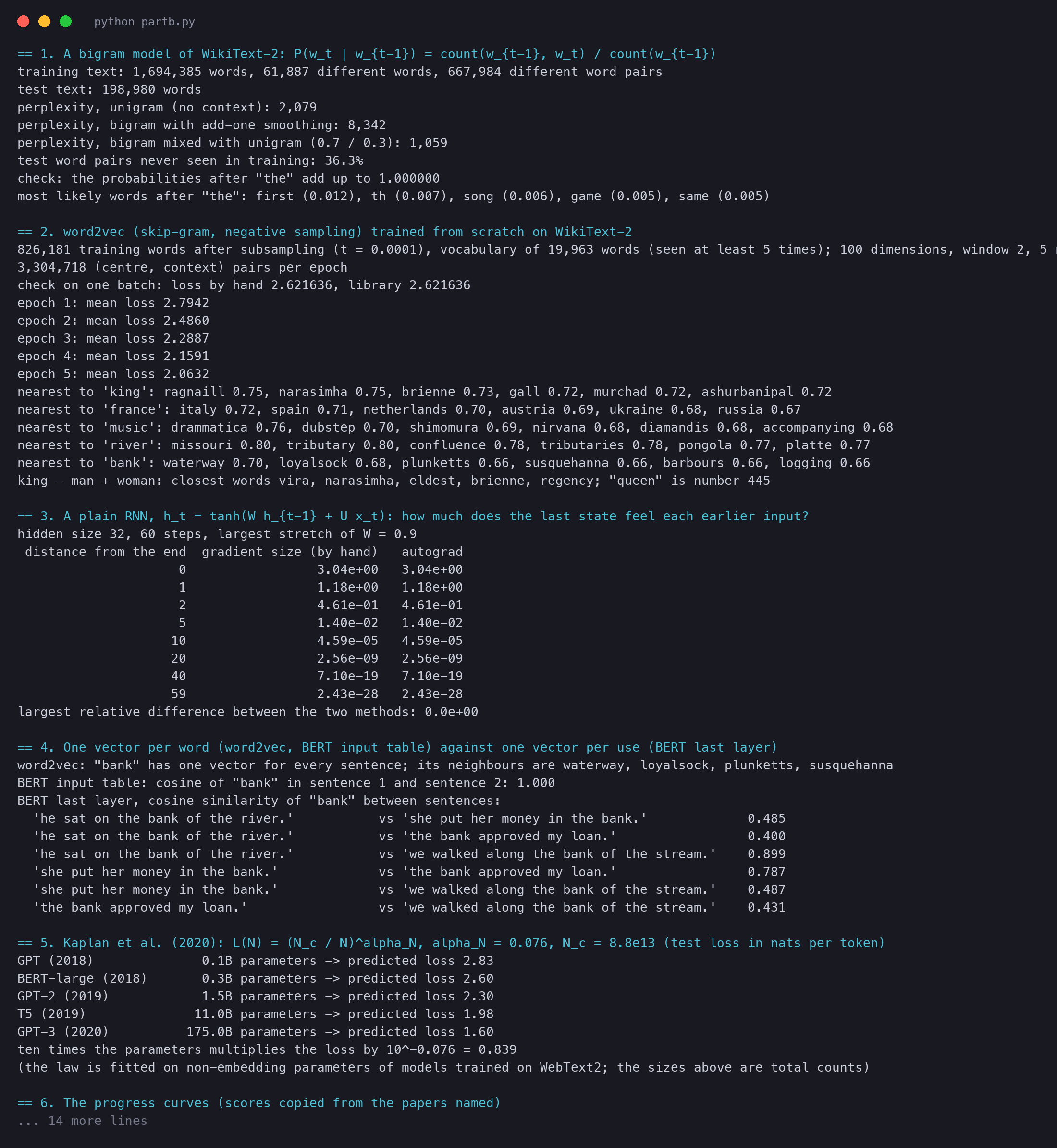
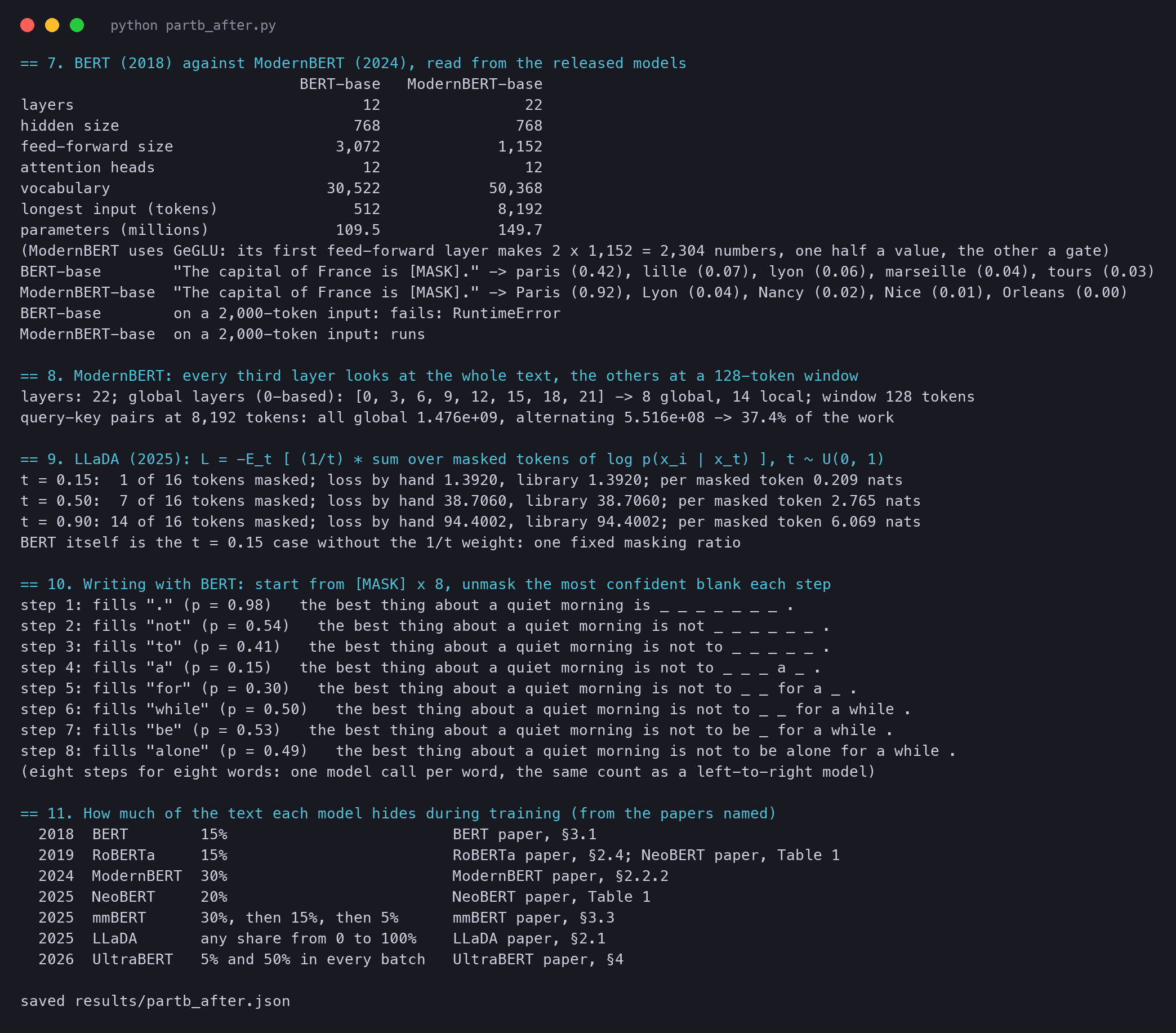
The full output of bert_partb.py, as it ran for this page.The full output of bert_partb_after.py.
## The papers
Before BERT: [word2vec](https://arxiv.org/abs/1301.3781) · [negative sampling](https://arxiv.org/abs/1310.4546) · [seq2seq](https://arxiv.org/abs/1409.3215) · [attention](https://arxiv.org/abs/1409.0473) · [Transformer](https://arxiv.org/abs/1706.03762) · [ULMFiT](https://arxiv.org/abs/1801.06146) · [ELMo](https://arxiv.org/abs/1802.05365) · [GPT](https://cdn.openai.com/research-covers/language-unsupervised/language_understanding_paper.pdf) · [GLUE](https://arxiv.org/abs/1804.07461) · [BERT](https://arxiv.org/abs/1810.04805)
After BERT: [SuperGLUE](https://arxiv.org/abs/1905.00537) · [RoBERTa](https://arxiv.org/abs/1907.11692) · [T5](https://arxiv.org/abs/1910.10683) · [scaling laws](https://arxiv.org/abs/2001.08361) · [GPT-3](https://arxiv.org/abs/2005.14165) · [DeBERTa](https://arxiv.org/abs/2006.03654) · [ModernBERT](https://arxiv.org/abs/2412.13663) · [NeoBERT](https://arxiv.org/abs/2502.19587) · [LLaDA](https://arxiv.org/abs/2502.09992) · [Ettin](https://arxiv.org/abs/2507.11412) · [mmBERT](https://arxiv.org/abs/2509.06888) · [UltraBERT](https://arxiv.org/abs/2610.15028) · [our scripts](https://github.com/ishwar6/ishwar-books/tree/main/code/papers/bert)