Circuits, explained · Part 1 of 1 · Covers Introduction, Model Simplifications, High-Level Architecture, Virtual Weights, Subspaces, Zero-Layer Transformers

The Big Idea and the Residual Stream

The opening of A Mathematical Framework for Transformer Circuits, read slowly: what mechanistic interpretability is, why the paper studies tiny attention-only models, the whole model written as four equations with every symbol and shape, the residual stream as a shared channel that layers read from and write to, virtual weights, the bandwidth problem, and why a zero-layer transformer can only learn bigrams. Every equation derived by hand, then checked on real models.

A Mathematical Framework for Transformer Circuits. Nelson Elhage, Neel Nanda, Catherine Olsson, Tom Henighan, Nicholas Joseph, Ben Mann, Amanda Askell, Yuntao Bai, Anna Chen, Tom Conerly, Nova DasSarma, Dawn Drain, Deep Ganguli, Zac Hatfield-Dodds, Danny Hernandez, Andy Jones, Jackson Kernion, Liane Lovitt, Kamal Ndousse, Dario Amodei, Tom Brown, Jack Clark, Jared Kaplan, Sam McCandlish, Chris Olah. Transformer Circuits Thread, 2021.

A trained language model is a big pile of numbers. Even the small two-layer model we use in this part has 52 million of them. Nobody chose these numbers by hand: training found them. The model uses them to predict the next word, and it does this well. But if you ask "what rule did it learn?", the numbers do not say.

In December 2021, a team at Anthropic published a long web article, A Mathematical Framework for Transformer Circuits, that tried to read the rules out of the numbers. It took the smallest transformers it could, wrote them in a new but exactly equal way, and showed that each one is a sum of simple pieces you can read straight from the weights.

This part covers the paper's setup: what "mechanistic interpretability" means, which parts of a transformer the paper removes, the whole model in four equations, the residual stream that every layer reads from and writes to, and why a transformer with zero layers can only learn bigrams (word pairs).

Each idea follows the same pattern: the paper's own words as a highlighted screenshot in a teal box; a plain-English explanation, with a yellow box for every new word; the maths, derived one step at a time with a small example you can check by hand; and the same idea on a real model, with real code and its real output. The models are small public ones, run with the TransformerLens library on the CPU of an Apple M5 Pro (64 GB).

The paper#

A circuit is a small part of a network that does one understandable job, such as "after the word Barack, predict Obama". The word comes from earlier work on image models, the Distill Circuits thread, which found such parts inside an image network. A framework is a set of equations and names: the paper does not train a new kind of model, it writes the usual one in a different but equal form.

Why reverse-engineer a model?#

A compiler turns readable source code into a binary file that a computer runs but a person cannot read. If you only have the binary, you reverse engineer it: work back from the bytes to what the program does. A trained transformer is in the same place. Training is the compiler, the weights are the binary, and nobody ever wrote the source code. Mechanistic interpretability tries to recover it.

Why want this? The paper's answer is safety: if we could read the algorithm, we could explain known problems, find new ones, and perhaps foresee the problems of bigger models that do not exist yet.

Start with the smallest models#

Modern models are huge, so the authors "start with the simplest possible models and work our way up": transformers with two layers or fewer and only attention blocks. The plan is to find simple patterns in these toy models, then look for them in big ones (the follow-up paper, In-context Learning and Induction Heads, did that).

The paper's summary of results has one finding per model size:

• Zero layers: the model learns bigram statistics, readable straight from the weights (end of this part).
• One layer: a bigram model plus skip-trigrams, patterns "A … B C" where token A earlier and token B now make C more likely (Parts 2 to 4).
• Two layers: heads combine into induction heads, which continue a pattern seen earlier in the text (Parts 5 and 6).

The simplifications#

A normal transformer layer (GPT-2, for example) has layer normalization, attention heads, an MLP, and biases inside each. The paper keeps only the attention heads.

1. No MLP layers: the big change#

Why remove it. Attention heads raise new questions that studying them alone answers cleanly, and, honestly, MLPs were much harder to understand: their non-linear function breaks the "sum of pieces" picture.

What it costs. A lot, and the paper calls it "a major weakness". These models are toys: they learn real behaviours (bigrams, copying, induction), but real models have MLPs. Part 7 covers how later work went back to them.

2. No biases: a free change#

Why remove it. A bias can always be turned into one more column of weights. Add an extra input number that is always 1, and put the bias in the matching column:

Read it in words: multiplying the bigger matrix by the longer vector gives $W x$ (from the first columns) plus $b\times1$ (from the last column). Here $W$ is any weight matrix (say $m\times n$), $x$ is the input ($n$ numbers), $b$ is the bias ($m$ numbers), and the new matrix $[W\;b]$ is $m\times(n+1)$.

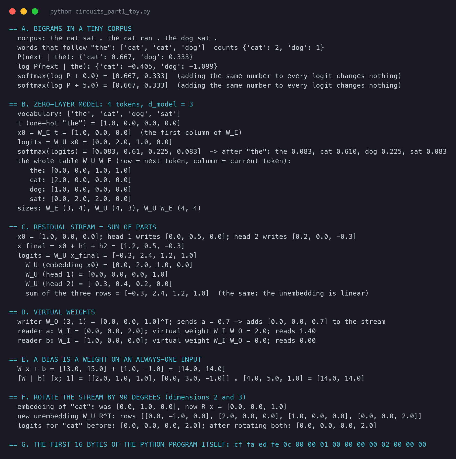
A tiny check from our toy script, with $W=\begin{bmatrix}2&1\\0&3\end{bmatrix}$, $b=(1,-1)$ and $x=(4,5)$:

What it costs. Nothing: a model with biases is a model without biases plus one always-1 dimension. The paper adds that in attention-only models the biases mostly act like a fixed bias on the final scores; we will see exactly that in the real model below.

3. No layer normalization: almost free#

Why remove it. The learned multiply-and-add part is linear, so it can be merged into the next matrix. What is left, "divide by the size", changes a vector's scale but not its direction: layer norm folds into nearby weights "up to a variable scaling".

What it costs. Very little. TransformerLens does this folding when it loads a model. We loaded attn-only-2l folded and unfolded, ran both on the same 31-token prompt, and compared every output log-probability:

== 2. FOLDING LAYER NORM INTO THE WEIGHTS
  prompt has 31 tokens; largest change in any log-probability after folding: 7.82e-05

A change of 0.00008 is rounding noise: the folded model is the same model. The division by the size cannot be folded, but it is one positive number per token, so it never changes which token scores highest.

The model in four equations#

Now the model itself. The paper studies autoregressive, decoder-only transformers like GPT-3: models that read text left to right and predict the next token. Here is the paper's own drawing.

We now go through the equations one at a time. The real model we use is attn-only-2l from TransformerLens: two layers, eight heads per layer, trained on web text and code in the style of the paper. Here are its sizes:

from transformer_lens import HookedTransformer
model = HookedTransformer.from_pretrained('attn-only-2l', device='cpu')
for name in ['W_E', 'W_pos', 'W_U', 'W_Q', 'W_K', 'W_V', 'W_O']:
    print(name, tuple(getattr(model, name).shape))

attn-only-2l: layers=2 heads/layer=8 d_model=512 d_head=64 n_vocab=48262 n_ctx=1024 attn_only=True params=52,094,086
  attn-only-2l W_E: (48262, 512)
  attn-only-2l W_pos: (1024, 512)
  attn-only-2l W_U: (512, 48262)
  attn-only-2l W_Q: (2, 8, 512, 64)
  attn-only-2l W_K: (2, 8, 512, 64)
  attn-only-2l W_V: (2, 8, 512, 64)
  attn-only-2l W_O: (2, 8, 64, 512)
  W_E + W_U hold 49,420,288 of 52,094,086 parameters

One warning. The paper writes vectors as columns ($W x$); TransformerLens writes them as rows ($x W$). So every TransformerLens matrix is the transpose of the paper's: the paper's $W_E$ is 512 × 48,262, TransformerLens stores 48,262 × 512. In the text we always use the paper's shapes. Notice also that 95% of the weights sit in the embedding and unembedding; the sixteen heads are small.

Equation 1: the embedding#

The model cannot do maths on words, so the first step turns each token into a vector of 512 numbers.

where:

• $t$ is the token, written as a one-hot vector: 48,262 numbers, all 0 except a single 1 at the token's index. Shape: $n_\text{vocab}=48{,}262$.
• $W_E$ is the embedding matrix, with one column per token. Shape: $d_\text{model}\times n_\text{vocab}=512\times48{,}262$.
• $x_0$ is the result: the token's starting vector in the residual stream. Shape: $d_\text{model}=512$.

Derivation. Why does multiplying by a one-hot vector give "the token's vector"? Write out the matrix-vector product for output number $i$:

Every $t_j$ is 0 except $t_k=1$, where $k$ is our token. So every term of the sum is 0 except one:

That is true for every row $i$. So $W_E t$ is simply column $k$ of $W_E$. The multiplication is a lookup.

Toy example. Take a vocabulary of four tokens (the, cat, dog, sat) and a stream of only 3 dimensions. Our toy script uses this $W_E$ (3 × 4), with one column per token:

Why write it this way, and what is it useful for? Code does a lookup, not a multiplication. The paper writes the multiplication on purpose: it makes the embedding a linear map like every other step, so it can be multiplied with later matrices. At the end of this part, the product $W_U W_E$ turns out to be a bigram table.

The real model also adds a position embedding from a 1024 × 512 table W_pos ("this is position 31"). The paper leaves it out of its equations, so we treat it as one more piece in our checks.

Equation 2: each layer adds to the stream#

where:

• $x_i$ is the residual stream vector before layer $i$. Shape: 512 (one such vector per token position).
• $H_i$ is the set of attention heads in layer $i$: eight heads in our model.
• $h(x_i)$ is what head $h$ computes from the stream. Shape: 512, the same as the stream, so it can be added.
• $x_{i+1}$ is the stream after the layer.

In words: every head reads the stream, computes something, and adds its result back. Nothing is overwritten or multiplied. The plus sign is the residual connection from ResNets. (A head also looks at the stream at earlier positions, which is what attention does; Part 2 covers that. Here we only need that its output is added.)

The paper's third equation, $x_{i+2}=x_{i+1}+m(x_{i+1})$, is the same "read, compute, add" for an MLP $m$. Attention-only models simply do not have it.

Equation 4: the unembedding#

where:

• $x_{-1}$ is the stream after the last layer (index $-1$ means "the last one", as in Python). Shape: 512.
• $W_U$ is the unembedding matrix, with one row per token. Shape: $n_\text{vocab}\times d_\text{model}=48{,}262\times512$.
• $T(t)$ is a vector of logits, one score per token in the vocabulary. Shape: 48,262. ($T$ for "transformer": the whole model is the function $T$.)

Toy example. In our 3-dimensional toy, take this $W_U$ (4 × 3), one row per possible next token:

With no layers at all, $x_{-1}=x_0=(1,0,0)$, the vector of "the". Each logit is one row of $W_U$ times that vector:

The softmax turns these scores into probabilities. The four exponentials are $e^0=1$, $e^2=7.389$, $e^1=2.718$ and $e^0=1$, which add up to 12.107. Dividing each by 12.107:

  logits = W_U x0 = [0.0, 2.0, 1.0, 0.0]
  softmax(logits) = [0.083, 0.61, 0.225, 0.083]  -> after "the": the 0.083, cat 0.610, dog 0.225, sat 0.083

So this toy model says: after "the", the next word is "cat" with probability 0.61.

What it is useful for. The unembedding is linear too. So if the stream is a sum of pieces, the logits are the same sum of pieces. The next section uses this.

Here is the whole real model in one picture, with the paper's shapes.

The residual stream as a communication channel#

Derivation: the stream is a sum#

The paper's claim follows from Equation 2 by writing it out. Take our two-layer model. Layer 0 gives

Layer 1 gives

Now replace $x_1$ in the second line by the right side of the first line:

That is the whole proof. The final stream is the embedding plus the output of every head, each added once. In the real model there are also the position embedding and one output bias per layer, so the final vector at one position has $1+1+8+1+8+1=20$ pieces.

Why this is special. In most networks the output of one layer goes through a non-linear function before the next layer sees it, so the pieces cannot be pulled apart. In the transformer, nothing is ever applied to the stream itself; layers only add to it. Even ResNets apply non-linear functions on their residual path.

Toy example. In our 3-dimensional toy, say head 1 writes $(0,0.5,0)$ and head 2 writes $(0.2,0,-0.3)$:

Now apply the unembedding. Because $W_U$ is linear, $W_U(a+b+c)=W_U a+W_U b+W_U c$, so the logits split into one piece per writer:

What it is useful for. If the logits are a sum, you can ask which piece pushed which token up. In the toy, "cat" gets 2.4: 2.0 from the token itself, 0.4 from head 2. This is called direct logit attribution.

Check it on the real model#

Now test both claims on attn-only-2l. The prompt is the opening sentence of a well-known novel, cut off halfway through a name it has already used: "Mr and Mrs Dursley, of number four, Privet Drive, were proud to say that they were perfectly normal. Mr and Mrs Durs". We split the stream at the last position into its 20 pieces and add them up (a shortened version of circuits_part1.py):

logits, cache = model.run_with_cache(tokens)       # run once, keep every inner signal
pos = tokens.shape[1] - 1                          # the last position ("urs")
parts = [cache['hook_embed'][0, pos], cache['hook_pos_embed'][0, pos]]
for L in range(2):
    z = cache[f'blocks.{L}.attn.hook_z'][0, pos]   # [8, 64]: each head's result vector
    for h in range(8):
        parts.append(z[h] @ model.W_O[L, h])       # what head L.h writes: 512 numbers
    parts.append(model.b_O[L])                     # the layer's output bias
real = cache['blocks.1.hook_resid_post'][0, pos]   # the real final stream vector
print((sum(parts) - real).abs().max())

In words: run_with_cache runs the model once and keeps every inner signal. The first two pieces are the token and position embeddings. For each head, hook_z holds its 64-number result, and multiplying by its output matrix W_O gives the 512 numbers it writes (Part 2 explains W_O). Each layer also adds a bias b_O. Finally we compare the sum with the real vector.

== 3. THE RESIDUAL STREAM AT THE LAST POSITION, TAKEN APART (attn-only-2l)
  last tokens: ['.', ' Mr', ' and', ' Mrs', ' D', 'urs']  -> model predicts 'ley'
  top 5: 'ley' 0.988, 'leys' 0.005, 'ki' 0.000, 'y' 0.000, 'a' 0.000
  20 parts; |sum of parts - real residual vector| max = 2.38e-06; ||x_final|| = 21.37
  first 4 coordinates of the real vector: [-0.256, -0.06, -0.569, -0.621]
  first 4 coordinates of the sum:         [-0.256, -0.06, -0.569, -0.621]

The model finishes "Dursley" ("ley", probability 0.988), and the 20 pieces add up to the real vector with a largest difference of 0.0000024: rounding noise. The stream really is a sum.

Now split the logit of "ley". One detail: before the unembedding, what is left of the last layer norm is "subtract the mean, divide by the size". Subtracting the mean is linear, so we apply it to each piece; the size is one number for the whole vector (0.945 here), so we divide every piece by it. Each piece's share is

where $W_U[\,:,\text{ley}\,]$ is the unembedding direction of "ley". The shares plus the unembedding bias add up to the real logit:

  sum of all lines = 20.645; the model's real logit = 20.645

Head 1.6 does almost half of the work. Where is it looking?

  head 1.6 at the last position attends to: position 6 'ley' 0.65, position 0 '<|BOS|>' 0.33, position 7 ',' 0.00

It looks back at the "ley" that followed "urs" the first time, and pushes "ley" up: a head that continues a pattern seen earlier in the text. That is an induction head, the subject of Part 6, found here with nothing more than addition.

Linear and additive: the key property#

What does "no privileged basis" mean? The model never looks at single dimensions of the stream on their own: it only reads through matrices and writes by adding. So we can rotate the whole stream, rotate every matrix that touches it to match, and the output stays the same.

Derivation. Let $R$ be a rotation: a square matrix with $R^\top R=I$ (turning back undoes turning). Rotate the stream: $x'=R x$. A reader with matrix $W$ is replaced by $W'=W R^\top$. Then the reader sees

exactly what it saw before. A writer $W_O$ becomes $R\,W_O$. Every number in the stream changes; every output stays the same. (In our 3-dimensional toy, a 90-degree turn moves "cat" from $(0,1,0)$ to $(0,0,1)$, and its logits stay $(0,0,0,2)$.)

Real model. We rotated all 512 dimensions of attn-only-1l at random (keeping fixed the all-ones direction that layer norm uses), together with every matrix that reads or writes the stream:

== 7. ROTATE THE RESIDUAL STREAM (attn-only-1l)
  rotation is orthogonal: max |R R^T - I| = 1.3e-06; keeps ones: 8.6e-08
  every weight that touches the stream changed (mean |change| in W_E: 0.218)
  largest change in any output logit: 9.6e-05

What it is useful for. It is a warning: "dimension 7 of the stream" has no meaning of its own, since a rotated model with a different dimension 7 behaves identically. Study the matrices that read and write the stream, and their products.

Virtual weights#

Reading and writing, as equations#

Give every layer two matrices:

• an input matrix $W_I$ that reads: the layer's input is $W_I x$. Shape: $d_\text{in}\times d_\text{model}$.
• an output matrix $W_O$ that writes: the layer adds $W_O a$ to the stream, where $a$ is what the layer computed. Shape: $d_\text{model}\times d_\text{out}$.

(A head has three input matrices, $W_Q$, $W_K$ and $W_V$; for now they are all "input weights", and Part 2 separates them.)

Derivation: where virtual weights come from#

Let layer 1 write $W_O^1a^1$ into the stream. Later, layer 2 reads the stream. By the sum rule above, the stream it reads contains layer 1's output as one term:

Layer 2 multiplies this by its input matrix. Matrix multiplication spreads over a sum, so:

Look at the middle term: what layer 2 receives from layer 1 is $a^1$ times one matrix, $W_I^2W_O^1$. It acts like a direct wire from layer 1 to layer 2, though no such wire exists in the code. The paper calls it a virtual weight.

The 512-wide stream drops out of the shape. What is left connects layer 1's outputs straight to layer 2's inputs.

Toy example. One writer and two readers on our 3-dimensional stream. The writer has $W_O=(0,0,1)^\top$: it writes its single number into dimension 3. It sends $a=0.7$. Reader A has $W_I=(0,0,2)$: it reads dimension 3. Reader B has $W_I=(1,0,0)$: it reads dimension 1.

Reader A receives $2\times0.7=1.4$. Reader B receives 0: the virtual weight says these two layers never talk, without running anything.

Real model. In attn-only-2l, take head 0.0 (layer 0, head 0). In the paper's shapes it reads with $W_V$ (64 × 512) and writes with $W_O$ (512 × 64). A head in layer 1 reads with its own $W_V$ (64 × 512). The virtual weight from a layer-0 head to a layer-1 head is therefore 64 × 64, much smaller than either matrix:

V = model.W_V[1, h2].T @ model.W_O[0, h1].T    # paper's W_V (64 x 512) times paper's W_O (512 x 64)

== 5. READING, WRITING AND VIRTUAL WEIGHTS (attn-only-2l, paper notation: W_V is d_head x d_model)
  head 0.0 reads with W_V (64, 512) and writes with W_O (512, 64)
  W_O W_V is (512, 512) = 262,144 numbers, but its rank is only 64
  virtual weight W_V(1.h2) W_O(0.h1): shape (64, 64), one for each of the 64 head pairs
  largest size (Frobenius norm): head 0.2 -> head 1.6: 5.41; smallest: head 0.0 -> head 1.5: 1.16
  (raw sizes are not yet a fair score of how much two heads talk; Part 5 normalises them)
  the embedding as a "layer 0 writer": W_E is (512, 48262); head 0.0 reading it: W_V W_E is (64, 48262)

Three things to see. There is one 64 × 64 virtual weight for each of the 64 pairs of heads; Part 5 turns their sizes into a fair score. The embedding is a writer too: $W_V W_E$ says what head 0.0 reads about each of the 48,262 tokens. And a head's own write-after-read matrix $W_O W_V$ is 512 × 512 but has rank only 64, because everything passes through the head's 64 numbers. That is where Part 2 starts.

Subspaces and bandwidth#

Once a layer writes something, it stays "unless another layer actively deletes it". So the stream's dimensions act like memory, or bandwidth: a limited number of lanes every message must share.

We counted the same numbers for our models. "Head outputs" is the number of heads times 64 (each head computes 64 numbers before writing); "MLP neurons" is 3,072 per layer in GPT-2 small.

== 6. BANDWIDTH
  attn-only-2l: residual stream 512 dims; heads write 1024 dims in total; MLP neurons 0; ratio 2.0x
  gpt2: residual stream 768 dims; heads write 9216 dims in total; MLP neurons 36864; ratio 60.0x

The toy model is mildly crowded (2 times). GPT-2 small, a real 12-layer model, is already at 60 times, on the way to the paper's "100 times" for a 50-layer model.

(The paper also notes, in a footnote, that in large models the embedding uses only a fairly small part of the stream. Checking this needs bigger models than ours, so we leave it for Part 7.)

The bandwidth paragraph also says the model is "somehow communicating in superposition". The paper only names the idea; it became the subject of Toy Models of Superposition and of Part 7.

The zero-layer transformer#

Now we can read the first real result of the paper. It is short, and everything above was needed for it.

Derivation 1: the model is one matrix#

With no layers, Equation 2 never runs, so the last stream is the first stream: $x_{-1}=x_0$. Put Equation 1 into Equation 4:

The last step only moves the brackets, which is allowed for matrix products. So the whole model is a single matrix $W_U W_E$ applied to the one-hot token. The paper drops the $t$ and writes $T=W_U W_E$.

The shapes:

By the one-hot rule, multiplying by $t$ picks one column: column $a$ of $W_U W_E$ is the list of next-token logits when the current token is $a$. The matrix is a table with one row per next token and one column per current token: the shape of a bigram table.

Toy example. Our toy's table is $W_U W_E$ = (4 × 3)(3 × 4) = 4 × 4. The script computed it:

  the whole table W_U W_E (row = next token, column = current token):
     the: [0.0, 0.0, 1.0, 1.0]
     cat: [2.0, 0.0, 0.0, 0.0]
     dog: [1.0, 0.0, 0.0, 0.0]
     sat: [0.0, 2.0, 2.0, 0.0]

Check one column by hand: column "the" is $W_U(1,0,0)^\top$, the first column of $W_U$, which is $(0,2,1,0)$: the logits we computed for Equation 4. This toy table has learned "the → cat", "cat → sat" and "dog → sat".

Derivation 2: the best table is the log of the bigram probabilities#

Why does the paper say the best $W_U W_E$ is "the bigram log-likelihood"? Here is the reasoning in three steps.

Step 1: what training rewards. A language model is trained to make the real next token likely. For one current token $a$, the training loss is the average of $-\log q(b\mid a)$ over all the times a token $b$ followed $a$ in the training text. Here $q(b\mid a)$ is the model's probability for $b$, the softmax of column $a$.

Step 2: the best possible guess. Let $P(b\mid a)$ be the true fraction of times $b$ follows $a$ in the data. A standard fact of probability (Gibbs' inequality) says that the average of $-\log q$, taken over data drawn from $P$, is smallest when $q=P$. In words: the loss is lowest when the model's probabilities equal the real frequencies. So the best zero-layer model has

Step 3: undo the softmax. Which logits give those probabilities? Try $z_b=\log P(b\mid a)+c$ for any number $c$:

The $e^c$ cancels, and the probabilities in the bottom add up to 1. So the best column is the log of the bigram probabilities, plus any constant. That is what "bigram log-likelihood" means.

Toy example. Take the nine-word text "the cat sat . the cat ran . the dog sat .". The word "the" is followed twice by "cat" and once by "dog":

== A. BIGRAMS IN A TINY CORPUS
  corpus: the cat sat . the cat ran . the dog sat .
  words that follow "the": ['cat', 'cat', 'dog']  counts {'cat': 2, 'dog': 1}
  P(next | the): {'cat': 0.667, 'dog': 0.333}
  log P(next | the): {'cat': -0.405, 'dog': -1.099}
  softmax(log P + 0.0) = [0.667, 0.333]  (adding the same number to every logit changes nothing)
  softmax(log P + 5.0) = [0.667, 0.333]  (adding the same number to every logit changes nothing)

The best column for "the" holds $\log(2/3)=-0.405$ for "cat" and $\log(1/3)=-1.099$ for "dog" (and very negative numbers for unseen words). Adding 5 to both changes nothing, as Step 3 promised.

The catch. A full bigram table for our vocabulary has $48{,}262^2\approx2.33$ billion entries, but $W_U W_E$ passes through a 512-wide middle, so its rank is at most 512. It cannot hold an arbitrary table. That is why the paper says "approximate": the model stores the best low-rank version it can.

The direct path in a real model#

The term $W_U W_E$ is not only the zero-layer model. In every transformer the stream is "embedding plus everything the layers add", so the logits always contain $W_U x_0=W_U W_E t$: the token's embedding going straight to the unembedding. The paper calls it the direct path.

In a model with layers, heads can predict part of the bigram table, so the direct path holds a kind of "residual": pairs no general rule explains, like "Barack" followed by "Obama". Let us read it from the weights of the one-layer attn-only-1l: take one token's embedding, multiply by $W_U$, list the five highest of the 48,262 scores.

t = model.to_single_token(' Barack')
row = model.W_E[t] @ model.W_U          # 48,262 scores: "after ' Barack', which token?"
print(model.to_str_tokens(row.topk(5).indices))

No text is run through the model; this reads the weights only.

== 4. THE DIRECT PATH W_U W_E (top 5 "next tokens" from the token alone)
  attn-only-1l
       ' Barack' -> ' Obama', ' Hussein', 'lung', 'Obama', 'hurst'   (rank of the token itself: 33)
       ' United' -> ' States', ' Nations', ' Kingdom', ' Methodist', ' Arab'   (rank of the token itself: 2623)
          ' New' -> ' Zealand', ' York', ' Yorker', ' Orleans', ' Testament'   (rank of the token itself: 33197)
         ' Hong' -> ' Kong', 'wei', 'chen', 'qi', 'yang'   (rank of the token itself: 2794)
           ' Mr' -> ' Corbyn', 'unal', ' Modi', ' Putin', ' Trump'   (rank of the token itself: 9452)
    ' according' -> ' to', ' specific', ' logger', ' diligence', ' respective'   (rank of the token itself: 620)
          ' Los' -> ' Angeles', 'artan', ' Santos', 'opian', 'erville'   (rank of the token itself: 15214)

This is the paper's own example, found in a different model trained by different people: "Barack" → "Obama". The other rows are bigrams too: "United States", "New Zealand", "Hong Kong", "according to", "Los Angeles". After "Mr" come surnames from the news.

The unembedding is not the inverse of the embedding#

A footnote adds: although $W_U$ is called the "un-embedding", it should not be the inverse of $W_E$. If it were, $W_U W_E$ would be the identity matrix, and the direct path would predict "the next token repeats this one", which is rarely true of text. The output above agrees: "Barack" ranks only 33rd after itself, "New" 33,197th. Over 2,000 ordinary tokens, we compared GPT-2, which uses the same matrix to embed and unembed ("tied" weights):

  attn-only-1l: tokens 1000..2999, share whose top direct-path prediction is the token itself: 0.000
  gpt2: tokens 1000..2999, share whose top direct-path prediction is the token itself: 0.988

The untied toy never picks the token itself; tied GPT-2 does so 98.8% of the time, and must use its layers to undo it. The direct path is a clean bigram table only when $W_U$ is free to differ from $W_E$, as in the paper's models.

What it is useful for. This is the paper's method in miniature: a behaviour ("after Barack, say Obama") found by multiplying two weight matrices, with no input text, and read by a person. Part 3 shows every model in the paper splits into terms like this; Parts 4 to 6 read the others.

Next, in Part 2: one attention head, opened up: why heads are independent and simply add, how a head moves information between tokens, and how its four matrices collapse into two, the QK circuit $W_Q^\top W_K$ (where to look) and the OV circuit $W_O W_V$ (what to copy).

Run it yourself

The two scripts behind this part are circuits_part1.py (every real-model number: shapes, layer-norm folding, the residual stream split into parts, the direct path, virtual weights, bandwidth and the rotation test) and circuits_part1_toy.py (the hand-sized examples). The first one downloads attn-only-1l, attn-only-2l and gpt2 from Hugging Face the first time, then runs on the CPU in about 15 seconds.

TransformerLens 4 replaced the HookedTransformer class used here, so install a 3.x version:

bashCopy

pip install torch "transformer_lens<4"
python circuits_part1.py        # writes results/part1.json and results/part1_stdout.txt
python circuits_part1_toy.py    # writes results/part1_toy.json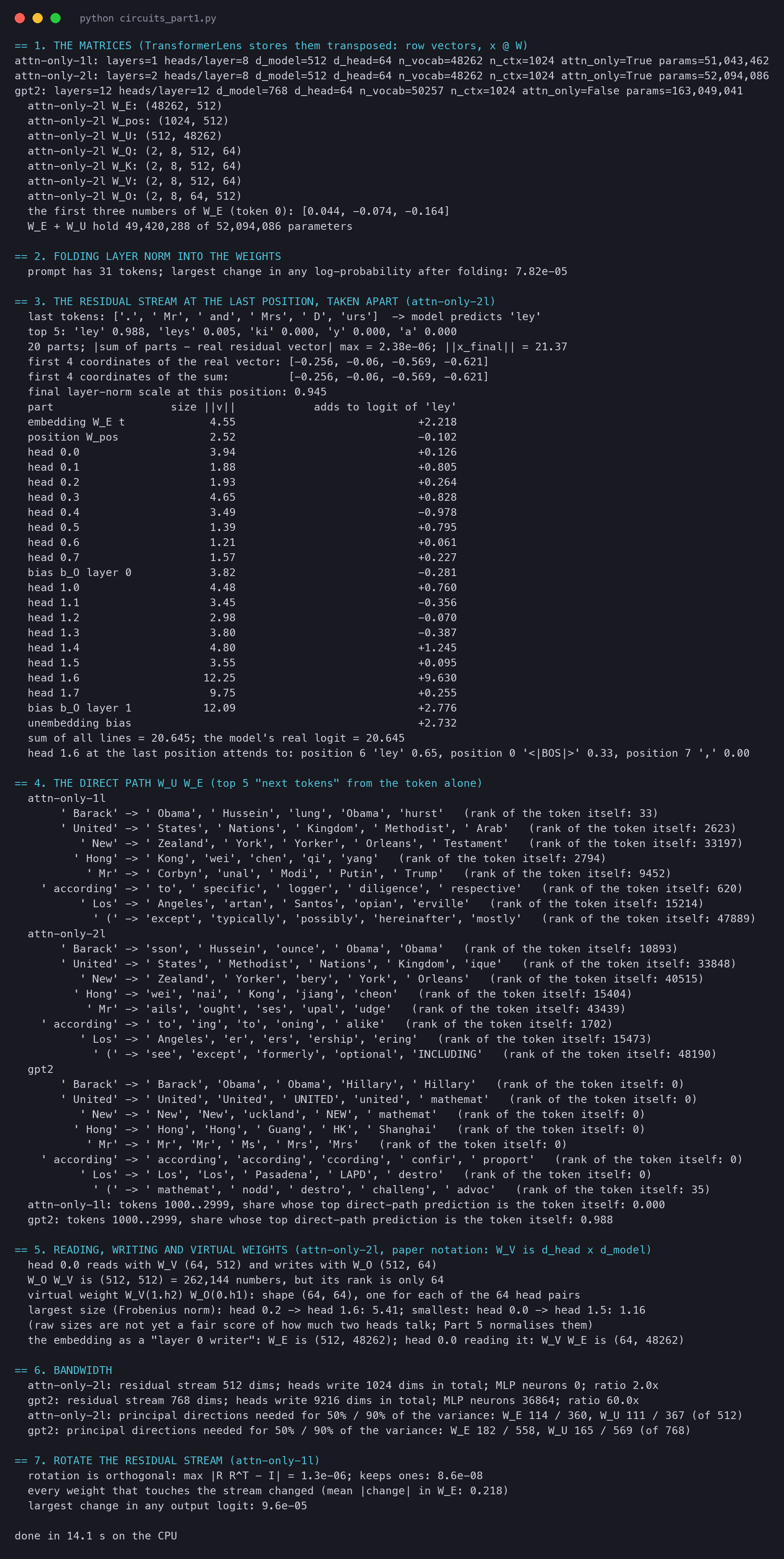

References#

The paper

1. N. Elhage, N. Nanda, C. Olsson, T. Henighan, N. Joseph, B. Mann, A. Askell, Y. Bai, A. Chen, T. Conerly, N. DasSarma, D. Drain, D. Ganguli, Z. Hatfield-Dodds, D. Hernandez, A. Jones, J. Kernion, L. Lovitt, K. Ndousse, D. Amodei, T. Brown, J. Clark, J. Kaplan, S. McCandlish, C. Olah. A Mathematical Framework for Transformer Circuits. Transformer Circuits Thread, Anthropic, 22 December 2021. The screenshots in this part come from this page.
2. Transformer Circuits Thread, the series of articles this paper opened.

Related papers

3. C. Olah, N. Cammarata, L. Schubert, G. Goh, M. Petrov, S. Carter. Zoom In: An Introduction to Circuits. Distill, 2020. Part of the Distill Circuits thread the paper builds on.
4. A. Vaswani, N. Shazeer, N. Parmar, J. Uszkoreit, L. Jones, A. N. Gomez, Ł. Kaiser, I. Polosukhin. Attention Is All You Need. NeurIPS 2017.
5. K. He, X. Zhang, S. Ren, J. Sun. Deep Residual Learning for Image Recognition (ResNet). CVPR 2016.
6. R. K. Srivastava, K. Greff, J. Schmidhuber. Highway Networks. 2015. The early residual-style network the paper mentions.
7. J. L. Ba, J. R. Kiros, G. E. Hinton. Layer Normalization. 2016.
8. T. B. Brown et al. Language Models are Few-Shot Learners (GPT-3). NeurIPS 2020.
9. A. Radford, J. Wu, R. Child, D. Luan, D. Amodei, I. Sutskever. Language Models are Unsupervised Multitask Learners (GPT-2). OpenAI, 2019.
10. O. Levy, Y. Goldberg. Neural Word Embedding as Implicit Matrix Factorization. NeurIPS 2014. The paper's footnote on embeddings as factorised log-likelihood tables.
11. C. Olsson, N. Elhage, N. Nanda, et al. In-context Learning and Induction Heads. 2022 (web version). The follow-up on large models.
12. N. Elhage, T. Hume, C. Olsson, et al. Toy Models of Superposition. 2022 (web version).

Tools and models

13. N. Nanda, J. Bloom, and contributors. TransformerLens, the library used for every experiment; version 3.9.0.
14. Model cards: NeelNanda/Attn_Only_1L512W_C4_Code (attn-only-1l), NeelNanda/Attn_Only_2L512W_C4_Code (attn-only-2l) and openai-community/gpt2.
15. Code for this part: circuits_part1.py and circuits_part1_toy.py.