How Meta-Harness found a way to look up solved problems for olympiad math, and a better harness for an agent that works in a terminal. We build the search engine and the discovered retriever in Python, test them with a small local model, and run two key pieces of the released agent code.
Meta-Harness: End-to-End Optimization of Model Harnesses. Yoonho Lee, Roshen Nair, Qizheng Zhang, Kangwook Lee, Omar Khattab, Chelsea Finn. COLM 2026, 2026. arXiv:2603.28052
The same search loop that wrote text classifiers in Part 3 gets two harder jobs here. In the first, it decides which solved problems a model sees before it attacks an olympiad problem. In the second, it changes the code around an agent that must finish long tasks in a terminal with no human help. Each piece below shows the exact lines of the paper, then explains them, and then rebuilds them in Python where a laptop can.
Here is the Jaccard test on a tiny pair. "find x if 2x = 10" has the word set {find, x, if, 2x, 10}. "find x if 2x = 12" has {find, x, if, 2x, 12}. They share 4 words, and together they have 6, so J=4/6=0.67. That is below 0.8, so the filter keeps the second problem. A short problem with one new number can pass the filter, which is why the authors also read the top search results by hand.
We cannot download the paper's corpus and test set at laptop scale, so we use a smaller public set with the same shape. MATH has 12,500 competition problems with full solutions. Each has a subject label (Algebra, Geometry, Number Theory and four more) and a difficulty level from 1 to 5. Its 7,500 training problems are our corpus, and its 5,000 test problems are our queries.
Our filter does both of the paper's tests. Exact prefix: the first 60 characters, in lower case. Fuzzy: the Jaccard similarity of the word sets, with the same 0.8 cut-off.
python
def words(text): return set(re.findall(r'\w+', text.lower()))def jaccard(a, b): return len(a & b) / max(1, len(a | b))def contaminated(query, corpus_words, word_postings, corpus_prefixes, n_prefix=60, thresh=0.8): """True if a corpus problem starts with the same 60 characters, or shares >= 80% of its word set. word_postings maps a word to the corpus problems that contain it, so we count shared words in one pass.""" if query[:n_prefix].strip().lower() in corpus_prefixes: return True q = words(query) shared = Counter(chain.from_iterable(word_postings.get(w, ()) for w in q)) # doc id -> |q & doc| return any(n / (len(q) + len(corpus_words[d]) - n) >= thresh for d, n in shared.items())
The last line uses a fact about sets: the size of the union is ∣A∣+∣B∣−∣A∩B∣. So once we count the shared words, we get the Jaccard similarity of every corpus problem without building a single union.
plain text
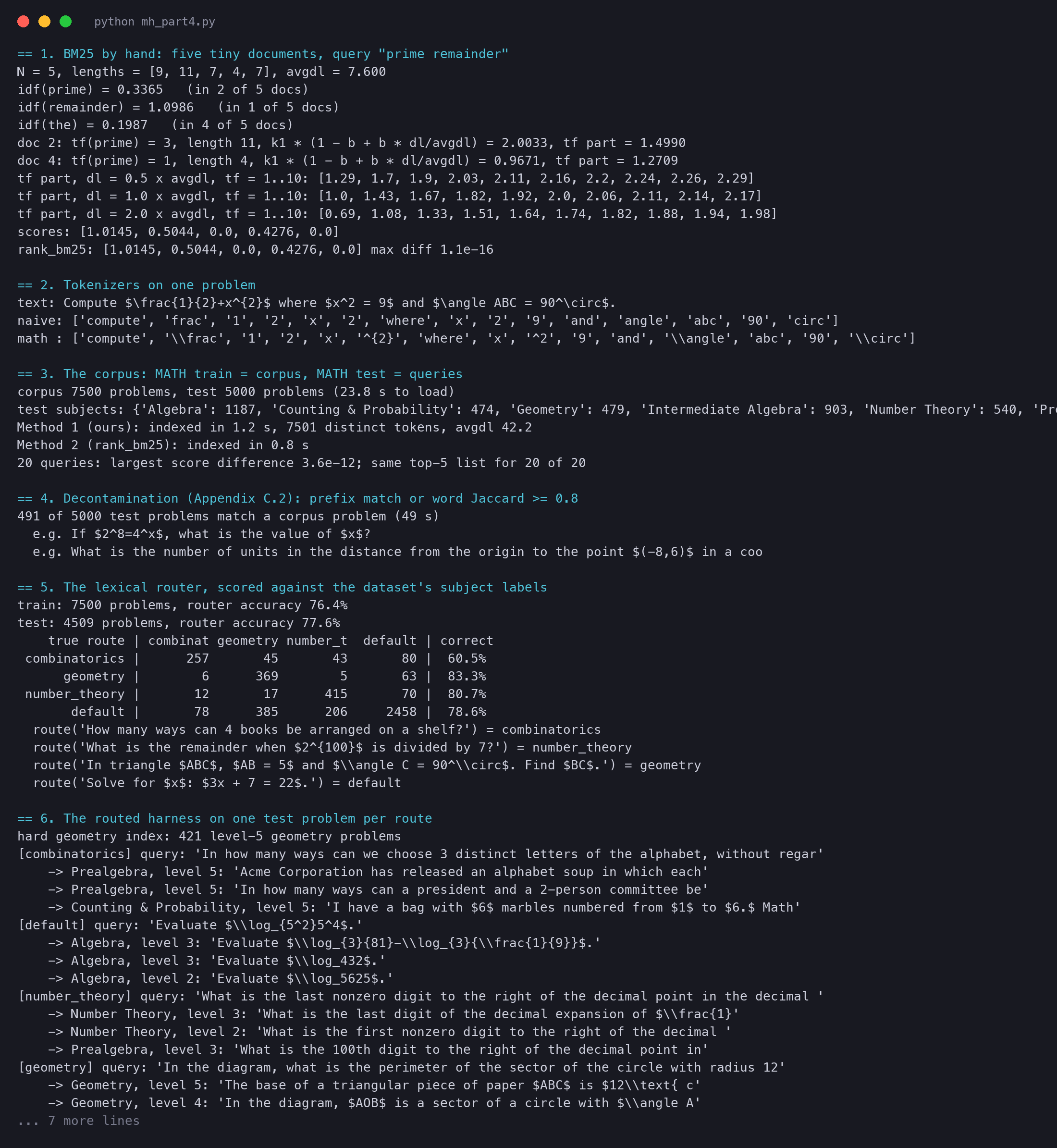
== 4. Decontamination (Appendix C.2): prefix match or word Jaccard >= 0.8491 of 5000 test problems match a corpus problem (49 s) e.g. If $2^8=4^x$, what is the value of $x$? e.g. What is the number of units in the distance from the origin to the point $(-8,6)$ in a coo
This surprised us. Almost one test problem in ten has a near copy in the training half of MATH. Without the filter, a retriever would fetch the answer for those 491 problems, and any score would look better than it is. Every experiment below uses only the 4,509 clean test problems.
Every harness in this section, the discovered one too, stands on one classic search method: BM25. It dates from the 1990s, and it is still the first thing to try when you search text by its words. It is worth understanding from the inside.
BM25 follows three common-sense rules. A rare word is better evidence than a common one: "remainder" tells you more than "the". A word that occurs more often in a document is better evidence, but the tenth time adds much less than the first. And a hit in a short document counts more than a hit in a long one, because a long document has many words by chance.
D is one document and Q is the query, a list of tokens. The score is a sum with one term for each query token q.
idf(q) is the inverse document frequency: how rare the token is. N is the number of documents, and n(q) is the number that contain q. A token in few documents gets a large idf.
f(q,D) is how many times q occurs in D, the term frequency.
∣D∣ is the length of D in tokens, and avgdl is the average length over the corpus.
k1 controls how fast extra hits stop helping. b controls how much length matters. The usual values are k1=1.5 and b=0.75.
When a token is in more than half the documents, the idf formula gives a negative number. The common library version then puts a small positive floor in its place: a quarter of the average idf. Our code does the same, so the two agree.
Take five tiny documents and the query "prime remainder":
"find the remainder when 100 is divided by 7" (9 tokens)
"the prime 7 and the prime 11 and the prime 13" (11 tokens)
"the radius of the circle is 6" (7 tokens)
"is 91 a prime" (4 tokens)
"the area of the square is 36" (7 tokens)
The average length is 38/5=7.6. "prime" is in 2 of the 5 documents, so idf=ln(3.5/2.5)=0.3365. "remainder" is in only 1, so idf=ln(4.5/1.5)=1.0986. The rare word is worth three times as much.
Document 1 has "remainder" once and 9 tokens. The length part is 1.5×(0.25+0.75×9/7.6)=1.7072. The term part is 2.5/(1+1.7072)=0.9235, and the score is 1.0986×0.9235=1.0145.
Document 2 says "prime" three times, in 11 tokens. Its term part is 7.5/(3+2.0033)=1.4990. Document 4 says "prime" once, but it is very short, so its term part is already 1.2709. Three hits beat one hit by only 18%. The score of document 2 is 0.3365×1.4990=0.5044, and document 4 gets 0.4276. Document 1 wins: one rare word beats three common ones.
The code builds an inverted index: for each token, the list of documents that contain it and how often. A query then only touches the documents that share a token with it, which is how real search engines stay fast.
python
def bm25_index(docs, k1=1.5, b=0.75, eps=0.25): """docs: a list of token lists. Builds what BM25 needs: idf per word, and postings (doc id, count) per word.""" N = len(docs) dl = [len(d) for d in docs] # document length in tokens avgdl = sum(dl) / N # average document length postings = defaultdict(list) # word -> [(doc id, term frequency in that doc)] for i, d in enumerate(docs): for w, f in Counter(d).items(): postings[w].append((i, f)) idf = {w: math.log((N - len(p) + 0.5) / (len(p) + 0.5)) for w, p in postings.items()} floor = eps * sum(idf.values()) / len(idf) # words in more than half the docs get a small positive idf idf = {w: (v if v >= 0 else floor) for w, v in idf.items()} return dict(N=N, dl=dl, avgdl=avgdl, postings=postings, idf=idf, k1=k1, b=b)def bm25_scores(ix, query): """BM25 score of every document for a query (a token list). Only docs that contain a query word get work.""" k1, b = ix['k1'], ix['b'] scores = [0.0] * ix['N'] for q in query: # a word repeated in the query counts each time for d, f in ix['postings'].get(q, []): norm = k1 * (1 - b + b * ix['dl'][d] / ix['avgdl']) # long documents need more hits scores[d] += ix['idf'][q] * f * (k1 + 1) / (f + norm) # saturates: the 10th hit adds little return scores
== 1. BM25 by hand: five tiny documents, query "prime remainder"N = 5, lengths = [9, 11, 7, 4, 7], avgdl = 7.600idf(prime) = 0.3365 (in 2 of 5 docs)idf(remainder) = 1.0986 (in 1 of 5 docs)idf(the) = 0.1987 (in 4 of 5 docs)doc 2: tf(prime) = 3, length 11, k1 * (1 - b + b * dl/avgdl) = 2.0033, tf part = 1.4990doc 4: tf(prime) = 1, length 4, k1 * (1 - b + b * dl/avgdl) = 0.9671, tf part = 1.2709tf part, dl = 0.5 x avgdl, tf = 1..10: [1.29, 1.7, 1.9, 2.03, 2.11, 2.16, 2.2, 2.24, 2.26, 2.29]tf part, dl = 1.0 x avgdl, tf = 1..10: [1.0, 1.43, 1.67, 1.82, 1.92, 2.0, 2.06, 2.11, 2.14, 2.17]tf part, dl = 2.0 x avgdl, tf = 1..10: [0.69, 1.08, 1.33, 1.51, 1.64, 1.74, 1.82, 1.88, 1.94, 1.98]scores: [1.0145, 0.5044, 0.0, 0.4276, 0.0]rank_bm25: [1.0145, 0.5044, 0.0, 0.4276, 0.0] max diff 1.1e-16
The scores are the ones we found by hand, and the library agrees to 10−16. "the" is in 4 of 5 documents, so its raw idf is negative and it gets the floor, 0.1987. The three "tf part" lines are the saturation rule in numbers; the chart shows them.
The term-frequency part of BM25 for 1 to 10 hits of one word, for a short, an average and a long document. The first hit adds the most. After about five hits the curve is almost flat, and it never goes above 2.5. At equal hits, the short document always scores higher.
On the full MATH corpus, the two methods also agree:
plain text
== 3. The corpus: MATH train = corpus, MATH test = queriescorpus 7500 problems, test 5000 problems (23.8 s to load)test subjects: {'Algebra': 1187, 'Counting & Probability': 474, 'Geometry': 479, 'Intermediate Algebra': 903, 'Number Theory': 540, 'Prealgebra': 871, 'Precalculus': 546}Method 1 (ours): indexed in 1.2 s, 7501 distinct tokens, avgdl 42.2Method 2 (rank_bm25): indexed in 0.8 s20 queries: largest score difference 3.6e-12; same top-5 list for 20 of 20
The paper says its BM25 index "uses a math-aware tokenizer that preserves LaTeX tokens (e.g., \frac, ^{2}) as atomic units". The reason is easy to see in code. A naive tokenizer keeps only letters and digits. The LaTeX command \frac becomes the word "frac", and the square in x^{2} becomes a lone "2" that looks like any other 2.
python
MATH_TOKEN = re.compile(r'\\[A-Za-z]+' # a LaTeX command: \frac, \sqrt, \angle r'|[\^_]\{[^{}]*\}' # a superscript or subscript group: ^{2}, _{10} r'|[\^_]\w' # a short one: ^2, _7 r'|\d+' # a number r'|[A-Za-z]+') # a worddef tokenize_math(text): """Math-aware tokens: every LaTeX command and every ^{...} or _{...} group stays one token.""" return [t if t.startswith(('\\', '^', '_')) else t.lower() for t in MATH_TOKEN.findall(text)]
With the math tokens, "squared" is its own token, and \angle is not confused with the English word "angle". On MATH the gain is small, as we show below. On a corpus of half a million problems, written in many LaTeX styles, the authors' search kept it.
The discovered harness: a router and four policies {Appendix B.2}#
The paper does not print its keyword lists, so we wrote our own: about 20 keywords per route and six regex cues for geometry notation. The full lists are in mh_part4.py. The router counts the cues of each route, and the route with the most cues wins.
python
GEOMETRY_REGEX = [r'\\angle', r'\\triangle', r'\\overline\{[A-Z]{2}\}', r'\\pi r', r'\b[A-Z]{3}\b', r'\b[A-Z]{2}\s*=\s*\d'] # notation such as triangle ABC, AB = 5def route(problem): """Count the cues of each route; the route with the most cues wins. No cue at all: the default route.""" text = problem.lower() hits = {r: sum(text.count(k) for k in ks) for r, ks in KEYWORDS.items()} hits['geometry'] += sum(len(re.findall(p, problem)) for p in GEOMETRY_REGEX) best = max(hits, key=hits.get) return best if hits[best] > 0 else 'default'
MATH gives us something the paper's test set does not: a subject label on every problem. So we can grade the router. Counting & Probability should go to combinatorics, Geometry to geometry, Number Theory to number theory, and the other four subjects to default.
plain text
== 5. The lexical router, scored against the dataset's subject labelstrain: 7500 problems, router accuracy 76.4%test: 4509 problems, router accuracy 77.6% true route | combinat geometry number_t default | correct combinatorics | 257 45 43 80 | 60.5% geometry | 6 369 5 63 | 83.3% number_theory | 12 17 415 70 | 80.7% default | 78 385 206 2458 | 78.6% route('How many ways can 4 books be arranged on a shelf?') = combinatorics route('What is the remainder when $2^{100}$ is divided by 7?') = number_theory route('In triangle $ABC$, $AB = 5$ and $\\angle C = 90^\\circ$. Find $BC$.') = geometry route('Solve for $x$: $3x + 7 = 22$.') = default
The confusion table of our router on 4,509 clean MATH test problems. Each row is the true route and adds up to 1; each column is the route the router chose. The diagonal is the share it got right. The largest error is in the bottom row: 385 algebra, precalculus and other problems went to geometry.
A keyword router gets about three problems in four right, and it is wrong in ways you can read. Many precalculus problems talk about angles and circles, so they go to geometry. A counting problem that never says "ways" or "probability" falls to default. A wrong route is not a disaster here, because every route still runs BM25 on the whole corpus. It changes how many examples come back and how they are sorted, not where they come from.
The four recipes of Figure 8 fit in one function. The paper does not give its weights or thresholds, so ours are our own choice. The rerank adds 0.15 for difficulty and 0.1 for a named technique. MATH's level (1 to 5) stands in for difficulty, and our hard geometry index holds the 421 level-5 geometry problems.
python
def retrieve(problem, ix, corpus, hard_geometry, tokenize=tokenize_math):
    """The routed harness: pick a route, then run that route's retrieval policy. Returns (route, doc ids)."""
    r = route(problem)
    scores = bm25_scores(ix, tokenize(problem))
    if r == 'combinatorics':                                      # BM25@20, dedup to 8, rerank, keep 3
        cands = dedup(top_k(scores, 20), corpus, keep=8)
        return r, rerank(cands, scores, corpus)[:3]
    if r == 'geometry':                                           # 1 hard reference + 2 raw BM25 neighbours
        hard = max(hard_geometry, key=lambda i: scores[i])
        return r, [hard] + [i for i in top_k(scores, 3) if i != hard][:2]
    if r == 'number_theory':                                      # BM25@12, rerank with a technique bonus, keep 3
        return r, rerank(top_k(scores, 12), scores, corpus, w_tech=0.1)[:3]
    cands = rerank(top_k(scores, 10), scores, corpus)             # default: BM25@10, rerank, adaptive K
    return r, cands[:adaptive_k(cands, scores)]
Here it is on one test problem of each route:
plain text
== 6. The routed harness on one test problem per routehard geometry index: 421 level-5 geometry problems[combinatorics] query: 'In how many ways can we choose 3 distinct letters of the alphabet, without regar' -> Prealgebra, level 5: 'Acme Corporation has released an alphabet soup in which each' -> Prealgebra, level 5: 'In how many ways can a president and a 2-person committee be' -> Counting & Probability, level 5: 'I have a bag with $6$ marbles numbered from $1$ to $6.$ Math'[default] query: 'Evaluate $\\log_{5^2}5^4$.' -> Algebra, level 3: 'Evaluate $\\log_{3}{81}-\\log_{3}{\\frac{1}{9}}$.' -> Algebra, level 3: 'Evaluate $\\log_432$.' -> Algebra, level 2: 'Evaluate $\\log_5625$.'[number_theory] query: 'What is the last nonzero digit to the right of the decimal point in the decimal ' -> Number Theory, level 3: 'What is the last digit of the decimal expansion of $\\frac{1}' -> Number Theory, level 2: 'What is the first nonzero digit to the right of the decimal ' -> Prealgebra, level 3: 'What is the 100th digit to the right of the decimal point in'[geometry] query: 'In the diagram, what is the perimeter of the sector of the circle with radius 12' -> Geometry, level 5: 'The base of a triangular piece of paper $ABC$ is $12\\text{ c' -> Geometry, level 4: 'In the diagram, $AOB$ is a sector of a circle with $\\angle A' -> Geometry, level 2: 'Two sectors of a circle of radius $12$ are placed side by si'
The examples are close in method. The logarithm question gets three logarithm questions. The decimal-digit question gets two problems about digits of a decimal expansion. The combinatorics route lifted two level-5 problems to the top, because of the difficulty bonus. Both are counting problems, even though MATH files them under Prealgebra.
One more test: how often do the retrieved examples come from the query's own subject? We ask this for 400 clean test problems.
plain text
== 7. Do the retrieved examples share the query's subject? (400 test problems) bm25 top-3 (naive tokens): 62.0% of retrieved examples share the subject bm25 top-3 (math tokens): 62.6% of retrieved examples share the subject routed harness: 62.8% of retrieved examples share the subjectrouted harness: 2.83 examples per problem on average (76 s for 400 queries x 3 methods)
The three numbers are almost the same. That is an honest result, and it teaches something. Plain BM25 already finds problems of the same subject most of the time, because the words give the subject away. The router does not change where the examples come from. It changes which of the near neighbours are shown, how hard they are, and how many. Whether that helps can only be measured by a model that reads them, as the paper does next.
The average column of Table 6, from the paper. Random few-shot falls below no retrieval. BM25 and five dense examples both help. The discovered harness has the highest average, 38.8%, 1.3 points above plain BM25.
We cannot run GPT-5.4 or Gemini, and IMO problems are far beyond a small local model. So we built the smallest honest copy of the experiment. The frozen model is Qwen2.5-1.5B-Instruct, with greedy decoding. The problems are 24 clean MATH test problems of levels 1 to 3, six from each route. Four harnesses fill the prompt: no retrieval, three random examples, BM25 top 3, and our routed harness.
The harness decides only what goes above the problem:
python
def build_prompt(problem, examples):
    """The harness's only job here: decide which solved examples go above the problem."""
    parts = []
    if examples:
        parts.append('Here are some solved problems that may help.\n')
        for ex in examples:
            parts.append(f'Problem: {ex["problem"]}\nSolution: {ex["solution"][:SOL_CHARS]}\n')
        parts.append('Now solve this problem.\n')
    parts.append(f'Problem: {problem}')
    return '\n'.join(parts)
plain text
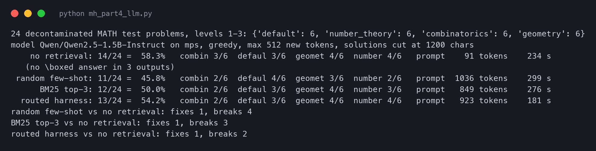
24 decontaminated MATH test problems, levels 1-3: {'default': 6, 'number_theory': 6, 'combinatorics': 6, 'geometry': 6}model Qwen/Qwen2.5-1.5B-Instruct on mps, greedy, max 512 new tokens, solutions cut at 1200 chars no retrieval: 14/24 = 58.3% combin 3/6 defaul 3/6 geomet 4/6 number 4/6 prompt 91 tokens 234 s (no \boxed answer in 3 outputs) random few-shot: 11/24 = 45.8% combin 2/6 defaul 4/6 geomet 3/6 number 2/6 prompt 1036 tokens 299 s BM25 top-3: 12/24 = 50.0% combin 2/6 defaul 3/6 geomet 4/6 number 3/6 prompt 849 tokens 276 s routed harness: 13/24 = 54.2% combin 2/6 defaul 3/6 geomet 4/6 number 4/6 prompt 923 tokens 181 srandom few-shot vs no retrieval: fixes 1, breaks 4BM25 top-3 vs no retrieval: fixes 1, breaks 3routed harness vs no retrieval: fixes 1, breaks 2
Our tiny copy of Table 6: accuracy of Qwen2.5-1.5B-Instruct on 24 clean MATH test problems with four harnesses. With so few problems, one problem is 4.2 points, so small differences are noise.
On our laptop, no harness beat the bare model. No retrieval solved 14 of 24 problems. Random examples solved 11, BM25 top 3 solved 12, and our routed harness solved 13. The last three lines count single problems. The routed harness fixed 1 problem and broke 2. BM25 fixed 1 and broke 3, and random examples fixed 1 and broke 4.
Two lessons hide in these small numbers. The first agrees with the paper: among the three ways to retrieve, the order is the same as in Table 6. Random examples hurt most, plain BM25 hurts less, and the routed policy hurts least. The second is a warning. A 1.5-billion-parameter model reads about 900 tokens of other solutions, and that distracts it more than it helps. The paper's models are much larger, and they can use a good example without being thrown off by it.
With 24 problems, one problem is 4.2 points, and a gap of one or two problems is within noise. We do not claim that our routed harness is better than BM25. We only show the machinery, and that a weak model can lose from retrieval. This is why the paper tests on five models. A policy is only useful if it does not hurt the model you happen to use.
The second experiment of this part is very different. The model no longer answers one question. It works as an agent. It types commands into a terminal, reads what comes back, and decides what to do next. It repeats this for many steps, until it thinks the task is done.
The Haiku 4.5 rows of Table 7, from the paper. Hand-written harnesses around the same model range from 13.9% to 35.5%. The harness that Meta-Harness found reaches 37.6%. The row "Anthropic's agent" is Anthropic's own coding agent, the same tool the paper uses as its proposer.
The discovered agent harness {Appendix B.3, Figure 9}#
The released harness is public: one file, agent.py, of 1,321 lines. It needs the Harbor framework and an API key to run, so we cannot run the agent. But the bootstrap is a shell command, and we can run that on a laptop. We copied the command from agent.py and changed only the folder name, so we can point it at a test folder.
python
# The command of AgentHarness._gather_env_snapshot, copied from agent.py. Only the folder name is a parameter.BOOTSTRAP = ( "echo '@@PWD@@' && pwd && " "echo '@@LS@@' && ls -la {app}/ 2>/dev/null && " "echo '@@LANG@@' && " "(python3 --version 2>&1 || echo 'python3: not found') && " "(gcc --version 2>&1 | head -1 || echo 'gcc: not found') && " "(g++ --version 2>&1 | head -1 || echo 'g++: not found') && " "(node --version 2>&1 || echo 'node: not found') && " "(java -version 2>&1 | head -1 || echo 'java: not found') && " "(rustc --version 2>&1 || echo 'rustc: not found') && " "(go version 2>&1 || echo 'go: not found') && " "echo '@@PKG@@' && " "(pip3 --version 2>&1 || echo 'pip3: not found') && " "(pip --version 2>&1 || echo 'pip: not found') && " "(apt-get --version 2>&1 | head -1 || echo 'apt-get: not found') && " "echo '@@MEM@@' && free -h 2>/dev/null | head -2 || true")
The @@PWD@@, @@LS@@ lines are markers. They split one long output into named sections. Method 1 is the parser of agent.py, rewritten in a few lines. A marker line opens a new section, and every other line goes into the open one. Method 2 does the same with one regular expression. The script checks that both give the same sections.
python
def parse_sections(stdout): """Method 1: the parser of agent.py. A line @@NAME@@ starts a new section; other lines go to the open one.""" sections, key, lines = {}, None, [] for line in stdout.split('\n'): if line.startswith('@@') and line.endswith('@@'): if key: sections[key] = '\n'.join(lines) key, lines = line.strip('@'), [] else: lines.append(line) if key: sections[key] = '\n'.join(lines) return sectionsdef parse_sections_re(stdout): """Method 2: one regular-expression split on the marker lines gives [before, NAME, body, NAME, body, ...].""" parts = re.split(r'^@@(\w+)@@$', stdout, flags=re.M) return {k: v.strip('\n') for k, v in zip(parts[1::2], parts[2::2])}
We run it twice. The first run uses a folder that holds three files, as a task folder would. The second uses a folder that does not exist.
plain text
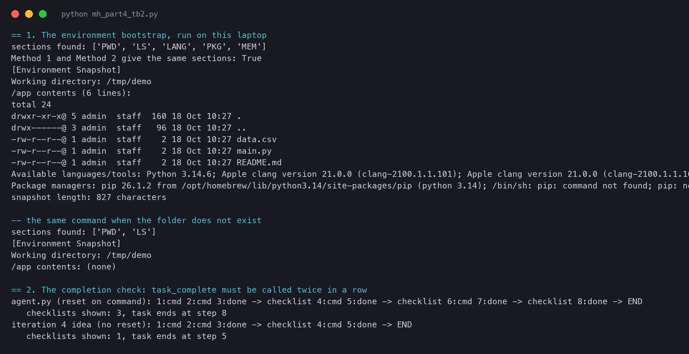
== 1. The environment bootstrap, run on this laptopsections found: ['PWD', 'LS', 'LANG', 'PKG', 'MEM']Method 1 and Method 2 give the same sections: True[Environment Snapshot]Working directory: /tmp/demo/app contents (6 lines):total 24drwxr-xr-x@ 5 admin staff 160 18 Oct 10:27 .drwx------@ 3 admin staff 96 18 Oct 10:27 ..-rw-r--r--@ 1 admin staff 2 18 Oct 10:27 data.csv-rw-r--r--@ 1 admin staff 2 18 Oct 10:27 main.py-rw-r--r--@ 1 admin staff 2 18 Oct 10:27 README.mdAvailable languages/tools: Python 3.14.6; Apple clang version 21.0.0 (clang-2100.1.1.101); Apple clang version 21.0.0 (clang-2100.1.1.101); v24.21.0; The operation couldn’t be completed. Unable to locate a Java Runtime.; rustc 1.96.1 (31fca3adb 2026-06-26); /bin/sh: go: command not found; go: not foundPackage managers: pip 26.1.2 from /opt/homebrew/lib/python3.14/site-packages/pip (python 3.14); /bin/sh: pip: command not found; pip: not found; /bin/sh: apt-get: command not foundsnapshot length: 827 characters-- the same command when the folder does not existsections found: ['PWD', 'LS'][Environment Snapshot]Working directory: /tmp/demo/app contents: (none)
The first run is what the model would read before its first turn: where it is, which files are there, and what it can use. On this laptop, Python, Node and Rust are present; Go and Java are not. An agent that reads this will not waste a turn trying go build.
The second run shows something we did not expect. The parts of the command are joined with &&, which means "run the next part only if this one succeeded". When ls fails because the folder is missing, every later part is skipped: no languages, no package managers, no memory. The || true at the very end only keeps the whole command from failing. The command assumes that the task files are in /app, as in TerminalBench-2, so this does not happen there. But it is a good example of a harness tuned to its benchmark: the same code in another setting would quietly report much less.
The checklist of Figure 9 has a small state machine. When the agent calls task_complete for the first time, the harness does not end the task. It shows the checklist ("Does your solution meet the requirements ... from the perspectives of a test engineer, a QA engineer, and the user") and sets a flag. Only a second task_complete right after ends the task. Any command in between clears the flag.
Appendix A.2 tells us that in iteration 4, the proposer wanted to delete the line that clears the flag. It saw agents that had solved a task but then ran a check command and lost the flag. They saw the checklist again and went round in circles for 30 to 60 steps. We replay both rules on the same sequence of actions:
python
def replay(actions, reset_on_command=True):
    """actions: 'cmd' (run commands) or 'done' (call task_complete). Returns the log and the step it ended on.
    agent.py: the first 'done' shows a checklist and sets pending; a second 'done' right after ends the task;
    any command in between sets pending back to False (the line that iteration 4 wanted to remove)."""
    pending, log = False, []
    for step, a in enumerate(actions, 1):
        if a == 'done':
            if pending:
                log.append(f'{step}:done -> END')
                return log, step
            pending = True
            log.append(f'{step}:done -> checklist')
        else:
            if reset_on_command:
                pending = False
            log.append(f'{step}:cmd')
    return log, None
plain text
== 2. The completion check: task_complete must be called twice in a rowagent.py (reset on command): 1:cmd 2:cmd 3:done -> checklist 4:cmd 5:done -> checklist 6:cmd 7:done -> checklist 8:done -> END checklists shown: 3, task ends at step 8iteration 4 idea (no reset): 1:cmd 2:cmd 3:done -> checklist 4:cmd 5:done -> END checklists shown: 1, task ends at step 5
With the rule of agent.py, an agent that checks its work after each checklist sees the checklist three times and ends at step 8. Without the reset, it ends at step 5, which looks like a clear win for the iteration 4 idea. But the search said otherwise: that candidate scored lower than the baseline.
Our reading is that the reset has a purpose. It makes the agent confirm right after its last change, not after some earlier state. Our replay shows the cost of the rule, and only the benchmark could show its value. The released harness keeps the reset.
Our math experiment has the shape of the paper's, but almost every number is smaller. Our corpus has 7,500 problems, not 535,356, and our questions are school competition problems, not IMO problems. Our model has 1.5 billion parameters, and the paper's models are far larger. Our policy was written by us from the paper's description, while the paper's was selected from 109 candidates by a 40-iteration search. Our results can show how each piece works. They cannot confirm or refute the 4.7-point gain.
For TerminalBench-2 we ran no agent at all. Each run needs paid API calls to Opus 4.6 or Haiku 4.5, and each task takes minutes in its own container. What we could do is read the released code and run its two key pieces as plain Python. The snapshot command and the completion rule are the same code that scored 76.4%; only the model and the sandbox are missing.