How Models Are Trained · Part 3 · Learning From Feedback

Chapter 7 · Reward models: turning preferences into a number

Reward models from the inside: why RLHF learns a reward instead of asking people every time, ratings against comparisons, the Bradley-Terry model derived from a noisy-judge story, the reward model loss and its gradient worked by hand, rankings, label noise and normalisation, the architecture (a language model with a one-number head), a real LoRA reward model trained on UltraFeedback, its accuracy, calibration and length bias, best-of-n overoptimisation against a stronger gold reward model, margins and ensembles, and process rewards.

Goal: by the end of this chapter you can explain why RLHF needs a learned reward, derive the Bradley-Terry model and the reward model loss from scratch and compute them by hand, describe exactly how a reward model is built from a language model, train one yourself on real preference data, measure how good it is (accuracy, calibration, length bias), watch it being over-optimised, and name the main defences. You will also have a trained reward model on disk, which Chapter 8 uses to train a policy with PPO.

7.1 Why learn a reward?#

Chapter 6 gave us the machinery of reinforcement learning for text. A policy (the language model) writes a response, the response gets a reward, and the policy gradient nudges the model so that high-reward responses become more likely. Chapter 6 used rewards that a few lines of code could compute: does the answer contain a number, what does a sentiment classifier say. For the thing we actually care about, "is this a good answer to this person's question?", there is no such rule.

The obvious fix is to ask people. That does not scale. A single PPO run on a small model samples hundreds of thousands of responses; InstructGPT's PPO dataset alone had 31,000 prompts, each answered many times during training. Nobody can read and score all of that, and even if they could, the policy would have to wait for them at every step.

So RLHF splits the job in two:

1. People judge a modest number of responses, once. Typically tens of thousands of comparisons, sometimes a million.
2. A model learns to predict those judgements. After that, it can score any number of new responses in milliseconds.

That second model is the reward model.

Chapter 2 told the story of how this idea arrived: Christiano et al. (2017) taught a simulated robot to backflip from 900 bits of human feedback, Ziegler et al. (2019) and Stiennon et al. (2020) moved it to text, and InstructGPT (Ouyang et al., 2022) made it the standard recipe. Chapter 3 showed how reward models are evaluated (RewardBench) and gave a first glimpse of reward hacking. This chapter opens the box. It answers four questions:

• What exactly is learned? A model of how people choose, the Bradley-Terry model, which turns choices into scores (Sections 7.2 to 7.4).
• What does the network look like? A language model with its output layer replaced by a single number (Section 7.5).
• How well does it work? We train one and measure it (Sections 7.6 to 7.9).
• What goes wrong when you optimise against it? Overoptimisation, and what people do about it (Sections 7.10 to 7.12).

A warning before we start. A reward model is a proxy. It is trained to agree with people on the kind of responses it saw during training. The policy we optimise will produce new kinds of responses, and it will search, hard, for the ones the reward model likes most. Everything in this chapter is about how good that proxy is, and how to keep the optimiser from exploiting where it is wrong.

7.2 What people are asked: ratings or comparisons#

There are two natural ways to collect human judgements of a response.

• Ratings (also called absolute or Likert scores): "How good is this answer, from 1 to 7?"
• Comparisons (pairwise preferences): "Here are two answers to the same question. Which is better?"

Almost every RLHF system trains its reward model on comparisons. Christiano et al. (2017) gave their reason in one sentence: "We found comparisons to be easier for humans to provide in some domains, while being equally useful for learning human preferences." Stiennon et al. (2020) asked labelers to compare two summaries; InstructGPT asked them to rank 4 to 9 answers; Llama 2 (Touvron et al., 2023) asked for a choice between two answers plus how strongly they preferred it ("significantly better", "better", "slightly better", "negligibly better or unsure").

Why would comparisons be better? Ratings carry more information per judgement: a rating of 6 against a rating of 3 says not only which is better but by how much. The problem is that each person uses the scale differently, and even one person's scale wanders. A strict rater's 5 is a lenient rater's 7. After reading three excellent answers, a decent one feels like a 4; after three bad ones, the same answer feels like a 6. A comparison is made with both answers side by side, at the same moment, by the same person, so whatever offset that person has at that moment cancels out.

That argument is easy to state and easy to over-sell, so let us test it with a small simulation. ch7_bt.py invents 200 answers with a hidden "true quality" and 20 raters. Each rater has a personal offset (harsh or generous) and a personal scale (uses a narrow or a wide range). Each rater sees 60 answers and either rates each one on a 1 to 10 scale (1,200 ratings in total) or compares them in 30 side-by-side pairs (600 comparisons in total). From the ratings we estimate quality by averaging; from the comparisons we fit a Bradley-Terry model (Section 7.3). Then we ask how well each estimate recovers the true order, measured by the rank correlation (1.0 means a perfect order). We run it three times: with raters whose offset is fixed, and with raters whose offset drifts from one answer to the next (a random walk with step 0.3 or 0.6), which is a simple model of the context effects just described.

200 answers, 20 raters (own offset and scale), each sees 60 answers: 1200 ratings or 600 comparisons; 50 repeats
  drift 0.0: rank correlation with the truth | mean rating 0.898 (sd 0.028) | Bradley-Terry 0.768 (sd 0.036) | comparisons better in 0/50
  drift 0.3: rank correlation with the truth | mean rating 0.777 (sd 0.059) | Bradley-Terry 0.763 (sd 0.041) | comparisons better in 18/50
  drift 0.6: rank correlation with the truth | mean rating 0.620 (sd 0.064) | Bradley-Terry 0.760 (sd 0.045) | comparisons better in 50/50

The result is more interesting than "comparisons are better":

• With stable raters, ratings win. Each rating says how good, not just which is better, and averaging two ratings per rater removes their offset anyway. Comparisons throw that magnitude away.
• With drifting raters, comparisons win. The Bradley-Terry estimate is the same 0.76 in all three settings: drift that hits both answers of a pair equally does not change which one looks better.

Real human judgement drifts, and real labeling teams are made of many people with different standards, so in practice comparisons are the safer choice. Many teams also collect a strength-of-preference grade or a rating alongside the comparison (Llama 2 does; InstructGPT also collected 1 to 7 quality scores as metadata), which recovers some of the lost magnitude. We will use exactly that in Section 7.11.

7.3 The Bradley-Terry model, derived#

We have comparisons: for prompt $x$, answer $y_w$ ("winner") was preferred to $y_l$ ("loser"). We want a function $r(x, y)$ that gives one number per answer. We need a bridge between the two: a statement of the form "if the scores are such and such, then a person picks $y_w$ with this probability". That bridge is a model of the judge.

Chapter 2 used the Bradley-Terry formula; Chapter 3 used it to rank chatbots. Here we derive it, because the derivation tells you exactly what a reward model assumes about people.

A noisy judge#

Imagine that each answer has a true quality $r$ and that, when a person looks at two answers, they perceive each quality with some noise: they see $r_w + \epsilon_w$ and $r_l + \epsilon_l$, where $\epsilon_w$ and $\epsilon_l$ are random, independent, and different every time. The person picks whichever looks better. Then

where:

• $y_w \succ y_l$ (read "$y_w$ is preferred to $y_l$") is the event that the person picks $y_w$;
• $r_w$ and $r_l$ are the true qualities (rewards) of the two answers;
• $\epsilon_w$ and $\epsilon_l$ are the person's perception noise for each answer.

The right-hand side depends on the qualities only through the gap $r_w - r_l$. The shape of the curve depends on the noise. Two classic choices:

• Normal noise gives the probit curve: this is Thurstone's model (1927), from psychology, built to explain judgements like "which of these two weights is heavier?".
• Gumbel noise (the distribution of the maximum of many random variables) has a neat property: the difference of two independent Gumbel variables follows the logistic distribution, whose cumulative curve is exactly the sigmoid. That gives

where:

• $\sigma$ is the sigmoid function, $\sigma(z) = 1/(1 + e^{-z})$;
• $e \approx 2.718$.

This is the Bradley-Terry model. Ralph Bradley and Milton Terry published it in 1952 in Biometrika for the analysis of "paired comparisons"; they wrote it as $P(i \succ j) = \pi_i / (\pi_i + \pi_j)$ with a positive "worth" $\pi_i$ for each item. Ernst Zermelo had found the same model in 1929 to rank chess players from incomplete tournaments. Set $\pi_i = e^{r_i}$ and divide top and bottom by $e^{r_i}$ and you get the sigmoid form above. The probit and logistic curves are nearly identical in shape; the logistic one is used because it is simpler to compute and its loss is the familiar cross-entropy.

What the reward gap means#

Turn the formula around. If $p = \sigma(r_w - r_l)$, then

where:

• $p$ is the probability that $y_w$ is preferred;
• $\frac{p}{1-p}$ is the odds of that preference (3 means "three times as likely to win as to lose");
• $\log$ is the natural logarithm.

So a reward gap is a log-odds. This is the sentence InstructGPT uses to describe Stiennon et al.'s loss: "the difference in rewards represents the log odds that one response will be preferred to the other by a human labeler." A gap of 0 means a coin flip; a gap of 1 means odds of $e^1 = 2.72$ to 1, a 73% chance; a gap of 2 means 88%; a gap of 4 means 98%.

Worked example. Our reward model gives the chosen answer 1.3 and the rejected one 0.4. The gap is 0.9, so the predicted chance that a person picks the chosen answer is $\sigma(0.9) = 1/(1 + e^{-0.9}) = 1/(1 + 0.4066) = 0.7109$. The odds are $0.7109 / 0.2891 = 2.46$, and $\log 2.46 = 0.9$: back to the gap.

The Elo link#

Chapter 3 met the same model as Elo ratings: a chess player with rating $R_A$ beats one with $R_B$ with probability $1 / (1 + 10^{-(R_A - R_B)/400})$. Since $10^{z} = e^{z \ln 10}$, this is $\sigma\big((R_A - R_B) \cdot \ln 10 / 400\big)$, the Bradley-Terry model with the scores multiplied by a constant. One unit of reward is worth $400 / \ln 10 = 173.7$ Elo points. Our gap of 0.9 would be a 156-point Elo gap. Going the other way, Chapter 3's example of a 100-point gap is a reward gap of $100 / 173.7 = 0.576$, and $\sigma(0.576) = 0.640$: the 64% Chapter 3 printed.

Elo: P = 1 / (1 + 10^(-(R_A - R_B) / 400)) = sigmoid((R_A - R_B) * ln(10) / 400)
so a reward gap of 1 equals 173.7 Elo points; our gap of 0.9 = 156 Elo points; 100 Elo points = gap 0.576 -> P 0.640

A reward model is therefore an Elo system for answers, with one important difference: Chatbot Arena fits one free number per model, while a reward model is a function. It must give a sensible score to answers it has never seen, from their text alone. That is what makes it useful, and what makes it fallible.

What the model assumes#

Writing the assumptions down helps later, when we see where reward models break:

1. One number per answer. All the things people care about (correctness, helpfulness, tone, safety, length) are collapsed into a single score. If two labelers weigh them differently, the model can only learn an average.
2. Independence from the alternative. How good $y_w$ is does not depend on what it is compared with.
3. Transitivity. If A usually beats B and B usually beats C, A must usually beat C. Real human preferences are not always transitive.
4. Noise of a fixed shape. Every comparison is equally noisy given the gap. In reality some labelers are careless and some pairs are genuinely ambiguous.

None of these is exactly true. All of them are close enough to be useful.

7.4 The reward model loss#

Now make the score a neural network with parameters $\theta$: $r_\theta(x, y)$. We have a dataset $D$ of comparisons $(x, y_w, y_l)$. Training means choosing $\theta$ so that the observed choices are as probable as possible under the Bradley-Terry model: maximum likelihood. The likelihood of the whole dataset is the product of $\sigma(r_\theta(x, y_w) - r_\theta(x, y_l))$ over all comparisons; taking minus the log turns the product into a sum, and dividing by the number of comparisons gives an average:

where:

• $\mathcal{L}(\theta)$ is the loss, a single number to minimise;
• $\theta$ are the reward model's parameters (for us, the LoRA weights and the score head);
• $\mathbb{E}_{(x, y_w, y_l) \sim D}$ means "the average over comparisons from the dataset $D$";
• $x$ is the prompt, $y_w$ the preferred ("chosen") response, $y_l$ the other ("rejected") one;
• $r_\theta(x, y)$ is the reward model's score for response $y$ to prompt $x$;
• $\sigma$ is the sigmoid and $\log$ the natural logarithm.

This is the loss of Stiennon et al. (2020), InstructGPT and Llama 2, written in nearly identical notation in all three papers. It is just binary cross-entropy where the "logit" is the reward gap and the label is always "the first one won".

Worked example: loss and gradient#

Take the pair from before: $r_\theta(x, y_w) = 1.3$ and $r_\theta(x, y_l) = 0.4$.

1. The gap is $1.3 - 0.4 = 0.9$.
2. $\sigma(0.9) = 0.7109$.
3. The loss is $-\log 0.7109 = 0.3412$.

If the model had them the wrong way round (gap $-0.9$), the loss would be $-\log \sigma(-0.9) = -\log 0.2891 = 1.2412$, almost four times bigger.

How does training change the rewards? Differentiate. Write $\Delta = r_w - r_l$ for the gap. Because $\frac{d}{d\Delta}\log\sigma(\Delta) = 1 - \sigma(\Delta)$,

where:

• $\Delta = r_\theta(x, y_w) - r_\theta(x, y_l)$ is the reward gap for one pair;
• $1 - \sigma(\Delta)$ is the probability the model currently gives to the wrong outcome.

Gradient descent moves each reward against its gradient: the chosen reward goes up, the rejected reward goes down, both by an amount proportional to $1 - \sigma(\Delta)$. For our pair that is $1 - 0.7109 = 0.2891$. A pair the model already gets right by a wide margin (gap 4, $1 - \sigma = 0.018$) barely moves anything; a pair it gets badly wrong (gap $-2$, $0.881$) gets almost the full push. The loss focuses the training on the mistakes.

# simplified from ch7_bt.py
t = torch.tensor([1.3, 0.4], requires_grad=True)     # r(chosen), r(rejected)
loss = -F.logsigmoid(t[0] - t[1])                     # the reward model loss for one pair
loss.backward()                                       # autograd computes the two derivatives

• F.logsigmoid computes $\log\sigma$ in one numerically safe step (computing sigmoid and then log separately overflows for large negative gaps).
• backward() fills t.grad with $\partial\mathcal{L}/\partial r_w$ and $\partial\mathcal{L}/\partial r_l$.

r(chosen) = 1.3, r(rejected) = 0.4, gap = 0.9
P(chosen beats rejected) = sigmoid(0.9) = 1 / (1 + e^-0.9) = 1 / (1 + 0.4066) = 0.7109
loss = -log(0.7109) = 0.3412
if the model had them the wrong way round (gap -0.9): P = 0.2891, loss = 1.2412
autograd: loss 0.3412, d loss / d r(chosen) = -0.2891, d loss / d r(rejected) = 0.2891
check: -(1 - P) = -0.2891
  gap -2: P 0.119  loss 2.127  gradient on r(chosen) -0.881
  gap -1: P 0.269  loss 1.313  gradient on r(chosen) -0.731
  gap +0: P 0.500  loss 0.693  gradient on r(chosen) -0.500
  gap +1: P 0.731  loss 0.313  gradient on r(chosen) -0.269
  gap +2: P 0.881  loss 0.127  gradient on r(chosen) -0.119
  gap +4: P 0.982  loss 0.018  gradient on r(chosen) -0.018

Note the value at gap 0: the loss is $\log 2 = 0.693$. A reward model that has learned nothing (gives every answer the same score) has exactly this loss. Every training log in this chapter should be read against 0.693.

Shifting every reward changes nothing#

Because only gaps appear, adding the same constant $c$ to every reward leaves the loss unchanged:

  shift   +0.0: rewards (1.3, 0.4) -> loss 0.3412
  shift  +10.0: rewards (11.3, 10.4) -> loss 0.3412
  shift   -7.5: rewards (-6.2, -7.1) -> loss 0.3412

The absolute level of a reward model's output is therefore arbitrary: training cannot fix it. That matters as soon as the reward is used. In PPO (Chapter 8) the reward is added to a KL penalty, so its level and scale interact with other terms. That is why every paper normalises the reward model after training: Christiano et al. normalised rewards "to have zero mean and constant standard deviation"; Stiennon et al. shifted them so reference summaries score 0; InstructGPT did the same with labeler demonstrations:

Rankings: K answers, K(K-1)/2 pairs#

InstructGPT made labeling cheaper by showing each labeler 4 to 9 answers at once and asking for a full ranking. A ranking of $K$ answers implies a comparison for every pair, $\binom{K}{2} = K(K-1)/2$ of them: 6 for $K = 4$, 36 for $K = 9$.

Worked example. A labeler ranks four answers A > B > C > D. The model currently scores them 2.1, 1.2, 0.9 and -0.5. The six pairs and their losses (from ch7_bt.py):

  A > B: gap +0.9, loss 0.3412
  A > C: gap +1.2, loss 0.2633
  A > D: gap +2.6, loss 0.0716
  B > C: gap +0.3, loss 0.5544
  B > D: gap +1.7, loss 0.1678
  C > D: gap +1.4, loss 0.2204
  mean over the 6 pairs (the 1/C(K,2) in InstructGPT's equation): 0.2698

(There is a more principled model for whole rankings, the Plackett-Luce model, which picks the best answer first, then the best of the rest, and so on. With $K = 2$ it reduces to Bradley-Terry. InstructGPT's sum over pairs is simpler and works well.)

Noisy labels#

People make mistakes. In the UltraFeedback data we will use, the labels come from GPT-4 and are noisier still. The plain loss treats every label as certain: if the model is confident (gap 10) that a label is wrong, the loss for that one pair is 10, and its gradient is nearly the maximum. A few mislabelled pairs can then dominate training.

Christiano et al. (2017) fixed this with a simple change to the judge model:

With a 10% chance of a random answer, the probability of the observed choice becomes

where:

• $0.1$ is the chance that the person answered at random;
• $0.5$ is the probability of either choice when answering at random;
• $0.9 \cdot \sigma(r_w - r_l)$ is the Bradley-Terry probability for the other 90% of judgements.

This probability can never go below 0.05 or above 0.95, so the loss of a pair can never exceed $-\log 0.05 = 3.0$:

  gap  1: plain P 0.73106, loss if the label is flipped   1.31 | noisy P 0.7080, loss if flipped 1.23
  gap  3: plain P 0.95257, loss if the label is flipped   3.05 | noisy P 0.9073, loss if flipped 2.38
  gap  6: plain P 0.99753, loss if the label is flipped   6.00 | noisy P 0.9478, loss if flipped 2.95
  gap 10: plain P 0.99995, loss if the label is flipped  10.00 | noisy P 0.9500, loss if flipped 2.99
  the flipped-label loss can never exceed -log(0.05) = 3.00

Modern reward models usually skip this and rely on one epoch of training (so no pair is seen twice) and on cleaner data. But the idea is worth knowing: the loss is a statement about how reliable you think your labels are.

7.5 Inside a reward model#

What network computes $r_\theta(x, y)$? It has to read a prompt and a long response and understand both well enough to judge quality. The thing that understands text best is a pretrained language model, so every modern reward model starts from one.

Recall from Chapter 4 that a language model is a stack of Transformer layers that turns each token into a hidden vector (896 numbers for Qwen2.5-0.5B), followed by an output head, a linear layer that maps each hidden vector to 151,936 scores, one per vocabulary token. A reward model keeps the stack and throws away the output head. In its place goes a score head, a linear layer from 896 numbers to 1.

Three details matter.

Which token. The Transformer produces a hidden state for every token, but we need one number for the whole response. Because attention is causal, the hidden state at the last token is the only one that has seen the entire prompt and response, so the score is read there. Our chats end with the <|im_end|> token that closes the assistant's turn. When several chats of different lengths are padded into one batch, the code must find each chat's last real token, not the last padding token; in Hugging Face's AutoModelForSequenceClassification this is done by searching for the last token that is not the pad token, which is why we set pad_token_id explicitly.

Which starting model. Stiennon et al. and InstructGPT start from the SFT model. Llama 2 starts from the chat model itself:

How big. InstructGPT used 6B reward models to train a 175B policy; Llama 2 used reward models the same size as the policy (7B to 70B). Stiennon et al. found that reward model accuracy improves steadily with both data and size:

7.6 The data: UltraFeedback#

For a real reward model we need real preference data. Two public datasets are widely used:

• Anthropic HH-RLHF (Bai et al., 2022): about 160,000 human comparisons of chat assistant replies, collected for helpfulness and harmlessness. The comparisons are human, but most replies are short and many conversations are multi-turn.
• UltraFeedback (Cui et al., 2023): about 64,000 prompts, each answered by 4 different models (from LLaMA-2 and Falcon to GPT-4), and each answer rated by GPT-4 for instruction following, truthfulness, honesty and helpfulness, plus an overall score from 1 to 10. The team behind Zephyr (Tunstall et al., 2023) turned it into pairs: the answer with the highest overall score is "chosen", one of the other three, picked at random, is "rejected". That version, UltraFeedback binarized, is a standard benchmark dataset for reward models and DPO.

We use UltraFeedback binarized, for three reasons: it is single-turn and varied, the answers come from many different models (so the reward model sees a range of quality), and it keeps both ratings, which we need for the margin loss in Section 7.11. Its labels come from GPT-4, not from people, so strictly this is RLAIF (RL from AI feedback, Chapter 2): our reward model learns to imitate GPT-4's judgement. The method is identical.

ch7_data.py loads it and keeps pairs that fit our budget:

UltraFeedback binarized train_prefs: 61,135 rows; ties (same rating) 12.1%
train: 4000 pairs | rating gap mean 2.21, median 1.50 | response tokens chosen 155, rejected 136 | chosen is longer in 53.1%
test: 600 pairs | rating gap mean 2.19, median 1.50 | response tokens chosen 155, rejected 139 | chosen is longer in 53.3%

• We drop ties: 12.1% of rows have the same rating for both answers, so there is no preference to learn.
• We keep pairs whose whole chat fits in 512 tokens, to keep training fast. This drops the longest answers, so our answers are shorter than in the full dataset.
• The rating gap (chosen rating minus rejected rating) has a median of 1.5 points out of 10: many pairs are close calls.
• The chosen answer is longer in 53% of pairs, and on average 19 tokens longer. Hold on to that number.

The test set is 600 pairs from UltraFeedback's own test split, never used in training. Here is one of them:

And this is exactly what the reward model reads for the chosen answer, the whole chat in Qwen's template:

'<|im_start|>system\nYou are Qwen, created by Alibaba Cloud. You are a helpful assistant.<|im_end|>\n<|im_start|>user\nComplete the sentence by providing an appropriate word. She was wearing a ____ dress.<|im_end|>\n<|im_start|>assistant\nThe word "red" would be an appropriate word to fill in the blank in the sentence "She was wearing a [___] dress."<|im_end|>'
... 74 tokens; last token id 151645 = <|im_end|>

The system line is added by Qwen's chat template when no system message is given. We drop the final newline that the template would add after <|im_end|>, so the last token, where the reward is read, is the one that closes the reply.

7.7 Hands-on: training a reward model#

Everything is in place: a backbone, a head, a loss and data. ch7_train.py trains the reward model; ch7_common.py holds the pieces it shares with the other scripts. We go through them block by block.

Building the model#

# simplified from ch7_common.py
BACKBONE = 'Qwen/Qwen2.5-0.5B-Instruct'

def build_rm(r=16, alpha=32, dropout=0.05):
    m = AutoModelForSequenceClassification.from_pretrained(BACKBONE, num_labels=1)
    m.config.pad_token_id = tok.pad_token_id          # <|endoftext|>: how the model finds each chat's last token
    cfg = LoraConfig(r=r, lora_alpha=alpha, lora_dropout=dropout, task_type='SEQ_CLS',
                     target_modules=['q_proj', 'k_proj', 'v_proj', 'o_proj', 'gate_proj', 'up_proj', 'down_proj'],
                     modules_to_save=['score'])        # the new head is trained in full
    return get_peft_model(m, cfg)

• AutoModelForSequenceClassification(..., num_labels=1) loads the pretrained transformer and adds the score head, a fresh $896 \times 1$ linear layer. The loading report says so: score.weight | MISSING ... newly initialized. The language model head is not loaded at all.
• pad_token_id is set so that, in a padded batch, the model reads the reward at each chat's last real token.
• The LoraConfig is the one from Chapter 5: rank 16 adapters on all seven linear layers of each of the 24 Transformer blocks. modules_to_save=['score'] tells LoRA to train the head itself rather than adapt it; it is new, so there is nothing to keep frozen.

The parameter count is a good check that we understand the model:

trainable parameters 8,799,104 of 502,832,768 (1.75%)

Per block, a rank-16 adapter on a layer of shape $d_{in} \times d_{out}$ adds $16 \cdot (d_{in} + d_{out})$ numbers. The query and output projections are $896 \times 896$ (28,672 each), key and value are $896 \times 128$ (16,384 each, Qwen shares keys and values across heads), and the three MLP layers connect 896 and 4,864 (92,160 each). That is 366,592 per block, $\times 24 = 8{,}798{,}208$, plus 896 for the head: 8,799,104.

One training step#

# simplified from ch7_train.py
for s in range(steps):                                        # 400 steps of 8 pairs = 3,200 pairs, one epoch
    batch = [train[i] for i in order[s * 8:(s + 1) * 8]]
    for k in (0, 4):                                          # two micro-batches of 4 pairs
        mb = batch[k:k + 4]
        ids, att = pad([p['ids_c'] for p in mb] + [p['ids_r'] for p in mb])   # 4 chosen + 4 rejected chats
        with torch.autocast('mps', dtype=torch.bfloat16):
            r = model(input_ids=ids, attention_mask=att).logits[:, 0].float()  # 8 rewards
        rc, rr = r[:4], r[4:]
        loss = -F.logsigmoid(rc - rr).mean()                  # the Bradley-Terry loss
        (loss / 2).backward()                                 # accumulate gradients over the 2 micro-batches
    torch.nn.utils.clip_grad_norm_(model.parameters(), 1.0)
    opt.step(); sched.step(); opt.zero_grad()

• Each step uses 8 pairs. They are split into two micro-batches of 4 pairs so that memory stays small; the gradients of the two are added up before the update (gradient accumulation, Chapter 4).
• pad puts the 4 chosen and the 4 rejected chats into one padded tensor of 8 rows, so one forward pass scores all of them. Lengths are rounded up to a multiple of 64 tokens: the GPU backend (all runs in this chapter are on an Apple M5 Pro, 64 GB) compiles its kernels once per tensor shape, and fewer distinct shapes means less waiting (the same trick as in Chapter 5).
• logits[:, 0] is the score head's output at each chat's last token: one reward per chat. The first 4 are the chosen answers, the last 4 the rejected ones, in the same order, so rc - rr gives the 4 gaps.
• torch.autocast(..., bfloat16) runs the matrix multiplications in 16-bit (Chapter 4, Section 4.10). It made steps about 30% faster in a quick test (2.5 against 3.5 seconds per step); the loss is computed in 32-bit.
• AdamW with learning rate $3 \times 10^{-4}$, a short linear warm-up (5% of the steps) then linear decay to zero, and gradient clipping at 1.0. (Why 3e-4 and not the more usual 1e-4 is explained below the run.)
• One epoch. Every paper we have quoted trains reward models for a single pass over the data: InstructGPT saw overfitting otherwise, and Llama 2 says "training longer can lead to over-fitting." We do the same.

Every 100 steps the script scores all 600 test pairs and records the accuracy: the share of pairs where the chosen answer gets the higher reward.

The run#

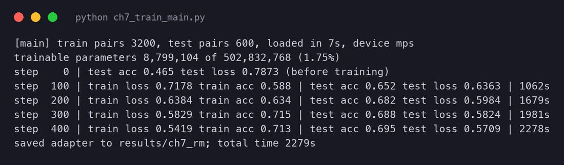
step    0 | test acc 0.465 test loss 0.7873 (before training)
step  100 | train loss 0.7178 train acc 0.588 | test acc 0.652 test loss 0.6363 | 1062s
step  200 | train loss 0.6384 train acc 0.634 | test acc 0.682 test loss 0.5984 | 1679s
step  300 | train loss 0.5829 train acc 0.715 | test acc 0.688 test loss 0.5824 | 1981s
step  400 | train loss 0.5419 train acc 0.713 | test acc 0.695 test loss 0.5709 | 2278s
saved adapter to results/ch7_rm; total time 2279s

How to read it:

• Before training the accuracy is 46.5%, not 50%. The new score head starts with random weights, so the untrained model already gives each answer an arbitrary score, by chance slightly anti-correlated with quality on this test set. Its loss, 0.787, is above 0.693 for the same reason: random scores are confidently wrong about half the time.
• Accuracy ends at 69.5% and rises only slowly after step 200. For a sense of scale (different data, so not a like-for-like comparison): Stiennon et al.'s 1.3B reward model agreed with labelers 62.4% of the time on summaries, and Llama 2's helpfulness reward model averages 63.2% on Meta's own test set.
• The test loss ends at 0.571. On the loss curve of Section 7.4, that means typical gaps are small: the model is rarely very confident. That is reasonable, since many pairs are close calls.
• Little overfitting. Training accuracy over the last 100 steps (71.3%) is close to test accuracy, as expected after one epoch.

The learning rate mattered more than anything else we tried. Our first run used $10^{-4}$, a common LoRA value. It is the lower curve in the figure: 52.8% after 100 steps and 62.7% at the end, with the same data, the same seed and the same schedule. Tripling the learning rate gave 69.5%. The plain Bradley-Terry loss gives small gradients once gaps open up (Section 7.4), so a reward model can under-train quietly; always compare a couple of learning rates on held-out pairs. Section 7.11 shows that this also changes how a margin loss looks.

The run took 38 minutes on the M5 Pro, including five passes over the test set. The adapter it saves, results/ch7_rm/, is 34 MB.

7.8 How good is it? Accuracy, calibration and scores#

ch7_eval.py loads the saved reward model (and the other reward models we trained, which Section 7.11 uses), scores all 600 test pairs, and looks at the results from several angles.

Accuracy, with an honest error bar#

main RM: accuracy 0.695 (95% bootstrap interval 0.657 to 0.732); mean loss 0.5709

With only 600 test pairs, 69.5% is uncertain by about 4 points either way. The interval comes from the bootstrap of Chapter 3, Section 3.6: resample the 600 pairs with replacement 2,000 times, recompute the accuracy each time, and keep the middle 95% of the results. Keep this in mind whenever two reward models in this chapter differ by a few points: on this test set, differences under about 4 points are within the noise.

Accuracy depends on how different the two answers are#

An average accuracy hides a lot. UltraFeedback keeps both GPT-4 ratings, so we can split the test pairs by the rating gap, exactly as Llama 2 split its test set by the labelers' strength of preference. We use four buckets with Llama 2's names: a rating gap below 1 is "negligibly better", 1 to 2 "slightly better", 2 to 4 "better" and 4 or more "significantly better".

by rating gap (chosen rating minus rejected rating):
  negligibly better     n=142  main 0.549  lr1 0.514  margin 0.556  seed1 0.542  seed2 0.563  small 0.585
  slightly better       n=192  main 0.672  lr1 0.615  margin 0.703  seed1 0.677  seed2 0.630  small 0.625
  better                n=136  main 0.779  lr1 0.654  margin 0.750  seed1 0.735  seed2 0.684  small 0.662
  significantly better  n=130  main 0.800  lr1 0.738  margin 0.785  seed1 0.777  seed2 0.731  small 0.754
  gold RM by rating gap: negligibly better 0.613, slightly better 0.760, better 0.838, significantly better 0.931

Our main model is right 80% of the time on clear cases and 55% on near-ties. The near-ties are not a failure of the reward model so much as a property of the data: if GPT-4's ratings differ by half a point, a different rater might well have ranked them the other way. Even the gold model, Skywork-Reward-V2 (a 2025 reward model of similar size, 0.6B parameters, but trained on far more and far cleaner preference data), manages only 61% there. Compare Llama 2's own numbers in Section 7.11: 80.7% on significantly better pairs, 54.7% on negligibly better ones. The shape is the same.

Calibration: does 80% mean 80%?#

The Bradley-Terry model makes a promise: when the reward gap is $\Delta$, the chosen answer should win with probability $\sigma(\Delta)$. A reward model that keeps this promise is calibrated. Calibration matters later: PPO treats reward differences as meaningful sizes, not just orderings.

To check, take each test pair's predicted probability $p = \sigma(r_w - r_l)$. The model's confidence in its own prediction is $\max(p, 1 - p)$ (it predicts whichever answer it thinks is likelier). Put the pairs into bins by confidence and compare, in each bin, the average confidence with the share of pairs the model got right:

  confidence 0.5 to 0.6: n=147  mean confidence 0.550  accuracy 0.483
  confidence 0.6 to 0.7: n=121  mean confidence 0.650  accuracy 0.620
  confidence 0.7 to 0.8: n= 98  mean confidence 0.750  accuracy 0.755
  confidence 0.8 to 0.9: n=108  mean confidence 0.851  accuracy 0.806
  confidence 0.9 to 1.0: n=126  mean confidence 0.955  accuracy 0.873
expected calibration error (ECE) 0.049

The summary number is the expected calibration error:

where:

• $B$ is the number of bins (5 here) and $b$ indexes them;
• $n_b$ is the number of pairs in bin $b$ and $N = 600$ the total;
• $\text{acc}_b$ is the share of pairs in the bin that the model got right;
• $\text{conf}_b$ is the model's average confidence in that bin.

Worked example with the table's values: $\frac{147}{600}\cdot 0.067 + \frac{121}{600}\cdot 0.030 + \frac{98}{600}\cdot 0.005 + \frac{108}{600}\cdot 0.045 + \frac{126}{600}\cdot 0.082 = 0.0164 + 0.0061 + 0.0008 + 0.0081 + 0.0172 = 0.0486$, which is the 0.049 the script prints.

An ECE of 0.049 is good for a model trained for one epoch on noisy labels. The pattern, overconfidence on the pairs it is surest about, is common: the most confident predictions include pairs where the label itself is wrong, which no reward model can get right. (This is the situation Christiano et al.'s 10% label-noise term was designed for.)

What the scores look like#

chosen   mean +5.317 sd 1.496 | rejected mean +4.427 sd 1.754 | gap mean +0.891 sd 1.668

Two things to notice. First, all rewards sit around +5, a level nobody chose: the loss never fixes it (Section 7.4), so it is wherever the random head and training happened to leave it. Second, the overlap. A good answer to a hard prompt can score lower than a bad answer to an easy one. A reward model ranks answers to the same prompt; comparing raw rewards across prompts mixes in how "rewardable" each prompt is. PPO's baseline and advantage (Chapter 6) remove exactly this per-prompt level, which is one reason they matter so much for RLHF.

For the example pair from Section 7.6, the model gives the chosen answer 4.20 and the rejected one 2.19: a gap of 2.01, so it is $\sigma(2.01) = 88\%$ sure the right answer won. It is.

7.9 What else did it learn? Length and other shortcuts#

A reward model learns whatever separates chosen from rejected answers in its training data. If chosen answers tend to be longer, length itself becomes a signal, whether or not people actually want longer answers. This is the most studied shortcut in reward modelling:

Recall from Section 7.6 that in our training data the chosen answer is longer in 53% of pairs. How much of that did the reward model absorb?

over all 1,200 test answers: corr(reward, length) Pearson 0.217 Spearman 0.147
                             corr(GPT-4 rating, length) Pearson 0.175 Spearman 0.124
within pairs: corr(reward gap, length gap) 0.205; corr(rating gap, length gap) 0.019
accuracy when the chosen answer is longer 0.762 (n=320), shorter 0.615 (n=273)

Read the three lines in order:

• Across all answers, longer answers get slightly higher rewards (Spearman 0.15), and GPT-4's ratings show about the same tilt (0.12). So far the reward model is just copying its labels.
• Inside a pair, which is what actually matters for training a policy, the picture changes. How much longer the chosen answer is barely predicts how much better GPT-4 rated it (0.02). But it predicts how much higher our reward model scores it (0.21). The model leans on length more than its labels justify.
• The accuracy split shows the same thing from another side: 76.2% when the chosen answer is also the longer one, 61.5% when it is the shorter one. Chapter 3 found the same asymmetry in published reward models on RewardBench (Skywork: 94% against 77%).

Correlation is not a test, though. A direct test is to take an answer, change only its length, and see what happens to the reward. ch7_eval.py does this with three edits on 150 chosen test answers, and asks the gold reward model the same question:

# simplified from ch7_eval.py
edits = {
    'add a polite closing line': lambda y: y + '\n\nI hope this helps! Let me know if you have any other questions.',
    'repeat the answer twice':   lambda y: y + '\n\n' + y,
    'cut the answer in half':    lambda y: ' '.join(y.split()[:len(y.split()) // 2]),
}
for name, f in edits.items():
    change = score(prompts, [f(y) for y in answers]) - score(prompts, answers)   # reward after minus before

  add a polite closing line  our RM: mean change -0.125 (sd of RM 1.35), up in 0.47 | gold RM: mean change -0.159 (sd 2.96), up in 0.43
  repeat the answer twice    our RM: mean change -0.119 (sd of RM 1.35), up in 0.35 | gold RM: mean change -1.966 (sd 2.96), up in 0.01
  cut the answer in half     our RM: mean change -2.526 (sd of RM 1.35), up in 0.01 | gold RM: mean change -4.282 (sd 2.96), up in 0.01

The edits tell a more useful story than the correlation:

• Cutting an answer in half is punished by both models, in 99% of cases; relative to its spread, ours punishes it even harder (1.9 standard deviations against 1.4). Our reward model does notice missing content.
• A polite closing line changes nothing much for either model: up in about half the cases, down in the other half.
• Repeating the whole answer is the revealing one. The gold model lowers the reward in 99% of cases, by two-thirds of a standard deviation: a repeated answer is obviously worse. Our reward model shrugs: an average change of $-0.12$, a tenth of its spread, and it actually raises the reward in 35% of cases. Doubling the length of an answer is nearly free.

That last line is the kind of hole an optimiser finds. PPO does not need the reward model to like repetition; it is enough that repetition is not punished while everything else that comes with longer answers is mildly rewarded. With 3,200 training pairs, almost none of which contain repeated text, our reward model has simply never been shown that repetition is bad. Section 7.10 shows this kind of gap between proxy and gold under real optimisation pressure.

7.10 Overoptimisation: when the proxy and the truth part ways#

A reward model is trained to rank answers like the ones in its training data. RLHF then uses it for something different: as a target to maximise. The optimiser searches for answers with the highest reward, and the highest-reward answers are disproportionately the ones where the reward model is wrong in the optimiser's favour. This is Goodhart's law ("when a measure becomes a target, it ceases to be a good measure") with a search algorithm attached. Chapter 3 introduced it under the name reward hacking; here we measure it.

Gao et al.: a gold reward model in place of people#

Measuring overoptimisation needs the true reward at every step of optimisation, which would mean asking people again and again. Gao, Schulman and Hilton (2022) used a trick: a large reward model plays the role of the people.

They optimised in two ways, best-of-n and RL (PPO), and measured how far the optimised policy had moved from the starting policy with the KL divergence (Chapter 1, Section 1.9). For best-of-n, the KL has an exact formula, so no estimate is needed:

where:

• $n$ is the number of samples best-of-n chooses from;
• $\text{KL}_{\text{bon}}$ is the KL divergence, in nats, between the distribution of the kept answer and the original policy's distribution.

For $n = 32$ this is $3.466 - 0.969 = 2.497$ nats. It grows only like $\log n$: to reach 10 nats you would need about $n = e^{11} \approx 60{,}000$ samples.

Their main finding is a pair of formulas for the gold reward as a function of the distance $d = \sqrt{\text{KL}}$:

For best-of-n:

where:

• $R_{\text{bon}}(d)$ is the gold reward gained over the starting policy ($R(0) = 0$);
• $d$ is the square root of the KL, a measure of how far optimisation has moved the policy;
• $\alpha$ is the initial slope: how much each unit of $d$ helps at first;
• $\beta$ is the rate at which the proxy's errors take over.

It is a downward parabola in $d$, with its peak at $d^* = \alpha / (2\beta)$. Optimising beyond $d^*$ makes the answers worse by the gold standard while the proxy keeps reporting progress.

The paper also measured how this depends on the proxy's training data:

Our version: best-of-32 against our reward model, judged by Skywork#

We cannot run Gao et al.'s full study, but we can run its best-of-n half in miniature, with our own reward model as the proxy and a much stronger public reward model as the gold.

• Policy: Qwen2.5-0.5B-Instruct, the model Chapter 8 will train.
• Prompts: 100 held-out UltraFeedback prompts (none of them in the reward model test pairs), with at most 150 tokens each.
• Samples: 32 answers per prompt, temperature 1.0, at most 256 new tokens (ch7_bon_gen.py). 3,200 answers in total; only 27.5% of them end within 256 tokens, the rest are cut off.
• Proxies: our main reward model (3,200 pairs), the small one trained on 400 pairs, and two ensembles (Section 7.11).
• Gold: Skywork-Reward-V2-Qwen3-0.6B, which scored 78.0% on our test pairs against our 69.5%.

One difference from Gao et al. matters: our proxy was trained on GPT-4's labels, not on the gold model's. So the gap between proxy and gold mixes two things, the proxy's errors and genuine disagreement between GPT-4's taste and Skywork's. Read the gold as "a second, better judge", not as the truth.

To get the expected reward of best-of-n for every $n$ from 1 to 32 from the same 32 samples, ch7_bon.py uses the estimator Gao et al. took from WebGPT (Nakano et al., 2021). Sort a prompt's $N = 32$ samples by proxy reward. The sample with rank $i$ (1 = lowest) is the best of a random subset of size $n$ exactly when the subset contains it and $n - 1$ of the $i - 1$ samples below it, so

where:

• $N = 32$ is the number of samples per prompt and $n$ the best-of-n size;
• $g_{(i)}$ is the gold reward of the sample with the $i$-th smallest proxy reward;
• $\binom{i-1}{n-1} / \binom{N}{n}$ is the probability that this sample is the one kept.

Worked example. For $n = 2$, the proxy's favourite ($i = 32$) has weight $\binom{31}{1} / \binom{32}{2} = 31 / 496 = 0.0625$, which is just $2/32$, the chance that it is one of the two drawn. The second-lowest sample ($i = 2$) has weight $1/496$: it is kept only if it is drawn together with the very lowest one. Averaging over all subsets this way is exact and has no sampling noise.

# simplified from ch7_bon.py
def bon(proxy, target, n):                       # proxy, target: arrays of shape (prompts, 32)
    tot = 0.0
    for p, t in zip(proxy, target):
        order = np.argsort(p)                     # samples from lowest to highest proxy reward
        w = np.array([math.comb(i, n - 1) for i in range(N)]) / math.comb(N, n)   # i = number of samples below
        tot += np.dot(w, t[order])
    return tot / len(proxy)

All rewards are first standardised (each model's rewards over the 3,200 samples get mean 0 and standard deviation 1), so proxy and gold are in comparable units, and each curve is measured from its value at $n = 1$.

proxy     n=1     n=2     n=4     n=8     n=16    n=32      (rewards in sd units, change from n=1)
main      proxy +0.000 +0.382 +0.667 +0.886 +1.058 +1.190
          gold  +0.000 +0.215 +0.377 +0.505 +0.618 +0.732
small     proxy +0.000 +0.419 +0.739 +0.962 +1.108 +1.206
          gold  +0.000 +0.095 +0.187 +0.276 +0.358 +0.433
gold      proxy +0.000 +0.384 +0.706 +0.975 +1.201 +1.384
          gold  +0.000 +0.384 +0.706 +0.975 +1.201 +1.384
KL(best-of-n || policy) in nats: 0.000 0.193 0.636 1.204 1.835 2.497

What we see:

• The gold still improves. Best-of-32 against our reward model raises the gold reward by 0.73 standard deviations. The proxy is not useless: picking what it likes helps.
• The proxy over-promises, more and more. At $n = 2$ the proxy claims +0.38 and the gold confirms +0.22, 56% of the claim. At $n = 32$ the claim is +1.19 and the gold confirms +0.73, 62%. In absolute terms the gap between the dashed and solid lines widens from 0.17 to 0.46. That widening gap is the beginning of overoptimisation.
• A weaker proxy over-promises much more. The 400-pair reward model promises almost the same (+1.21) but delivers +0.43, 36% of its claim. Its rankings within a prompt correlate only 0.21 with the gold's, against 0.52 for the main model.
• The ceiling. Using the gold model itself as the selector gives +1.38: that is what perfect agreement with the gold would buy at $n = 32$.
• No peak yet. Fitting Gao et al.'s form $d(\alpha - \beta d)$ to our gold curve gives $\alpha = 0.479$ and a $\beta$ of only 0.012: the curve is still almost a straight line in $d$. Our largest $n$ reaches a KL of 2.5 nats ($d = 1.58$), the far left of Gao et al.'s plots, where their gold curves also still rise. Seeing the turn-down by best-of-n alone would take thousands of samples per prompt. PPO travels much further in KL, which is why Chapter 8 needs a leash.

main: picks the gold favourite of 32 in 0.22 of prompts; mean within-prompt rank correlation with gold 0.517
small: picks the gold favourite of 32 in 0.13 of prompts; mean within-prompt rank correlation with gold 0.209

What does a disagreement look like? The prompt where our reward model's favourite was furthest below the gold's favourite asks for a question whose answer is "break up", given a passage about Pangaea:

  proxy pick: proxy +1.83, gold -0.05: 'Question: What happened at the end of the Mesozoic era when Pangaea broke apart? This question directly corresponds to the given answer "break up". It prompts the user to correctly identify the major '
  gold pick:  proxy +1.31, gold +2.61: 'Question: What phenomenon caused Pangaea to begin breaking apart millions of years ago?'

Our reward model prefers the answer that keeps talking, explaining its own question at length (and getting cut off); the gold model prefers the short question that does exactly what was asked. One example proves nothing, but it is the pattern Sections 7.8 and 7.9 predicted.

What best-of-n selects#

main      words  154.6  153.7  153.1  153.2  153.3  154.4
          done    0.27   0.31   0.35   0.38   0.43   0.47
gold      words  154.6  149.6  144.7  139.9  135.2  130.7
          done    0.27   0.32   0.36   0.40   0.45   0.53

Because three quarters of the samples are cut off, "did it finish?" dominates the selection here, and all selectors learn to prefer finished answers. The interesting difference is length: as $n$ grows, the gold model trades length away, our reward model does not. This is the length tilt of Section 7.9 seen under optimisation.

To check that cut-off answers are not the whole story, ch7_bon.py repeats the analysis using only finished answers, on the 35 prompts that have at least 8 of them (so $n$ goes up to 8):

finished answers only: 35 prompts with at least 8 finished answers (of 32)
main      proxy +0.000 +0.349 +0.585 +0.746 | gold +0.000 +0.199 +0.311 +0.390 | words 88 89 91 96
small     proxy +0.000 +0.100 +0.173 +0.227 | gold +0.000 +0.119 +0.189 +0.219 | words 88 86 84 82
gold      proxy +0.000 +0.394 +0.689 +0.919 | gold +0.000 +0.394 +0.689 +0.919 | words 88 80 73 70

Among finished answers the same picture holds: our reward model's picks gain 0.39 gold for 0.75 promised, and grow longer (88 to 96 words) while the gold model's picks grow shorter (88 to 70).

7.11 Defences: margins, ensembles and a leash#

No single trick removes overoptimisation, but several reduce it. We look at three, two of which we can test with the reward models we already trained.

Margins: using how strongly people preferred#

Llama 2 asked labelers not just which answer was better but by how much, on a four-level scale. Its reward model loss uses that grade:

where:

• $y_c$ and $y_r$ are the chosen and rejected responses (Llama 2's names for $y_w$ and $y_l$);
• $m(r)$ is the margin, a number that depends on the preference rating $r$ of the pair (here $r$ is the labeler's grade, not a reward);
• everything else is as in Section 7.4.

The loss is now small only when the gap exceeds the margin. For a pair with margin 3 and a gap of 0.9, the loss is $-\log\sigma(0.9 - 3) = -\log\sigma(-2.1) = 2.22$ instead of 0.34: the model is told that 0.9 is not enough for a "significantly better" pair.

The margins Llama 2 used, and what they gained:

The same paper reports how accuracy depends on how distinct the two responses are, which is a useful way to read any reward model's accuracy:

We trained a reward model with Llama 2's "margin large" (margins 0, 1, 2 and 3 for our four rating-gap buckets) and compared it with the plain loss at the same learning rate, data, seed and schedule ($10^{-4}$; Section 7.7 explained why our main model uses $3 \times 10^{-4}$):

  lr1     accuracy 0.627  reward sd 1.212
  margin  accuracy 0.697  reward sd 3.299
  main    accuracy 0.695  reward sd 1.690
  share of pairs with |reward gap| > 2: main 0.242, lr1 0.093, margin 0.538

At first sight the margin is a big win: 69.7% against 62.7%, far more than Llama 2's half a point. But look at the third line. The plain loss with a three times larger learning rate reaches 69.5%, the same accuracy. The margin helped here mostly by keeping the gradients large: subtracting a margin keeps $1 - \sigma(\Delta - m)$ big even after the model has the pair right, so the model keeps learning, much like a larger learning rate. Once the plain loss is tuned, the margin's advantage disappears within our error bar, which matches Llama 2's small ablation. By rating gap (the table in Section 7.8), the margin model is slightly ahead of the tuned plain model on the two closest buckets (55.6% against 54.9%, 70.3% against 67.2%) and slightly behind on the two clearest (75.0% against 77.9%, 78.5% against 80.0%); none of these differences is beyond the noise of 130 to 190 pairs per bucket.

What the margin reliably changes is the scale: the standard deviation of its rewards is 3.3 against 1.7, and 54% of test pairs get a gap above 2 against 24%. For RL that is not a detail: the reward's scale sets how strongly PPO pushes relative to its KL penalty (Chapter 8). It is one more reason rewards are normalised before RL.

Ensembles: several judges are harder to fool#

If several reward models are trained independently (different seeds, different data), they make different mistakes. An answer that exploits one of them is less likely to exploit all of them. Christiano et al. already averaged an ensemble in 2017. Coste et al. (2023) tested ensembles specifically against overoptimisation, in Gao et al.'s gold-model setup:

We have three reward models that differ only in seed and data shard: main, seed1 and seed2 (the last two trained on 1,600 pairs with $10^{-4}$, and therefore weaker). After scaling each to unit standard deviation, we combine them in two ways: the mean of the three rewards, and the minimum (Coste et al.'s worst case).

  ensemble (mean of main, seed1, seed2 after scaling each to unit sd) accuracy 0.690
  the three agree on 0.73 of pairs: accuracy there 0.732; where they disagree 0.577
  correlation of rewards over the 1,200 answers: main-seed1 0.68, main-seed2 0.36, seed1-seed2 0.59, main-margin 0.83, main-gold 0.60, small-gold 0.27

Three findings:

• The ensemble's accuracy (69.0%) is no better than its best member (69.5%). Averaging helps when members are about equally good and make independent errors. Ours are unequal: two weaker members dilute the strong one.
• Disagreement is informative. On the 73% of pairs where all three agree, the ensemble is right 73.2% of the time; where they disagree, 57.7%, little better than a coin. Disagreement between members is a cheap, useful signal of "the reward model does not know", which is exactly what uncertainty-weighted optimisation uses.
• The members are less alike than you would think. Trained on the same kind of data from the same backbone, two of them correlate only 0.36 across answers. Reward models are noisy functions; any single one has idiosyncrasies an optimiser can find.

Under best-of-n (same setup as Section 7.10):

ens_mean  proxy +0.000 +0.289 +0.513 +0.690 +0.832 +0.944
          gold  +0.000 +0.190 +0.340 +0.456 +0.533 +0.535
ens_min   proxy +0.000 +0.326 +0.576 +0.770 +0.924 +1.057
          gold  +0.000 +0.166 +0.291 +0.381 +0.433 +0.472

Here the ensembles deliver less gold than our main model alone (+0.54 and +0.47 against +0.73 at $n = 32$), and the mean's gold curve flattens between $n = 16$ and $n = 32$. That is not a contradiction of Coste et al.: their members were equally strong and they measured far deeper into optimisation, where a single proxy collapses. With members this unequal and optimisation this light, the honest summary is: ensembles are a defence against exploitation, not a way to make a better reward model, and they only pay off when you optimise hard. They also cost one forward pass per member at every step of RL.

The leash: a KL penalty#

The most widely used defence is not about the reward model at all. It limits how far the policy may move from where it started. Chapter 6 introduced the per-token KL penalty: the reward the policy actually maximises is

where:

• $r_\phi(x, y)$ is the reward model's score (we write $\phi$ for its parameters, to keep $\theta$ for the policy);
• $\pi_\theta$ is the policy being trained and $\pi_{\text{ref}}$ the frozen starting model;
• $\beta$ is the strength of the penalty;
• the log-ratio, averaged over responses, is the KL divergence between the two models.

In the language of this section, the KL term caps how far to the right on Gao et al.'s curves the policy can go: it keeps the policy where the reward model was trained, among answers that look like the starting model's, where its judgements are still meaningful. Gao et al. found that, in their RL setup, the penalty did not change the shape of the gold-versus-KL curve; it mostly stops the run earlier on it. Chapter 8 sets $\beta$ for our reward model and watches the KL during training.

Other defences, briefly: collect fresh comparisons on the current policy's outputs and retrain the reward model during RL (Llama 2 did this over five rounds, and Christiano et al. showed that offline-only reward models get exploited); penalise length explicitly or train a separate length head and discard it (for example ODIN, Chen et al., 2024); and, where answers can be checked, use a checker instead of a learned reward (Chapter 2's RLVR).

7.12 Process rewards: grading the steps, not just the answer#

Everything so far gives one reward for a whole response. For a multi-step maths solution that is a blunt signal: a solution with nine good steps and one slip gets the same low score as nonsense, and a solution that reaches the right number by a wrong argument gets full marks. A reward model that only sees outcomes is an outcome reward model (ORM). The alternative is to judge every step.

Uesato et al. (2022) compared the two on grade-school maths (GSM8K). Outcome supervision reached similar final-answer error rates with fewer labels, but to get the reasoning steps right they needed process-based feedback, or a reward model trained to imitate it. Lightman et al. (2023), in "Let's Verify Step by Step", scaled the idea up. They had people label every step of 75,000 solutions to 12,000 MATH problems as positive, negative or neutral: 800,000 step labels in all (the PRM800K dataset):

The PRM is a language model trained to predict, after each step, whether that step is correct. To compare solutions, it needs one number per solution:

As an equation:

where:

• $s$ is a solution made of $K$ steps;
• $p_k$ is the PRM's probability that step $k$ is correct;
• $\prod$ means "multiply together".

Worked example (illustrative step probabilities, computed by ch7_bt.py). A five-step solution where the PRM is confident in every step, $0.98, 0.96, 0.97, 0.95, 0.94$, scores $0.815$. A solution whose fourth step is wrong, $0.98, 0.95, 0.97, 0.30, 0.90$, scores $0.244$, although four of its five steps look fine. Taking the minimum step instead of the product gives 0.94 and 0.30, the same ordering.

== 7. process reward: scoring a solution from its steps (illustrative step probabilities) ==
  right answer    steps [0.98, 0.96, 0.97, 0.95, 0.94]: product 0.815, minimum 0.94
  one wrong step  steps [0.98, 0.95, 0.97, 0.3, 0.9]: product 0.244, minimum 0.30

How much better is it? Lightman et al. used best-of-N, as in Section 7.10, with each reward model picking the best of N sampled solutions:

Process rewards are expensive to label by hand, so later work generates step labels automatically (for example, by checking how often completions from a given step reach the right answer). And for problems with a checkable final answer, the field has also moved the other way: Chapter 2's RLVR and GRPO skip the learned reward model entirely and use the checker as the reward. Learned reward models remain essential wherever no checker exists: helpfulness, tone, safety, writing.

7.13 Saving the reward model for Chapter 8#

Chapter 8 trains Qwen2.5-0.5B-Instruct with PPO, and it needs a reward. It will use the main reward model from this chapter. ch7_train.py saved it with one line, model.save_pretrained('results/ch7_rm'), which writes only what was trained: the LoRA matrices and the score head (34 MB), not the 494 million frozen backbone weights. Loading it back:

# simplified from ch7_common.py (load_rm) and results/ch7_rm/README.md
base = AutoModelForSequenceClassification.from_pretrained('Qwen/Qwen2.5-0.5B-Instruct', num_labels=1)
base.config.pad_token_id = tok.pad_token_id                  # as in training: find each chat's last real token
rm = PeftModel.from_pretrained(base, 'results/ch7_rm').eval()

text = tok.apply_chat_template([{'role': 'user', 'content': prompt},
                                {'role': 'assistant', 'content': response}], tokenize=False).rstrip('\n')
reward = rm(**tok(text, return_tensors='pt')).logits[0, 0].item()

• from_pretrained(..., num_labels=1) rebuilds the same architecture: backbone plus a (randomly initialised) score head.
• PeftModel.from_pretrained loads the adapter on top and replaces the random head with the trained one, because the head was saved through modules_to_save.
• The text must be formatted exactly as in training: Qwen's chat template, final newline stripped, so the last token is <|im_end|>. A reward model is only reliable on inputs that look like its training data; a different template is a distribution shift.

Three things Chapter 8 has to handle, all of which this chapter has measured:

1. The scale is arbitrary. Section 7.4 showed the loss ignores shifts. Before RL, the rewards are normalised using samples from the starting policy, so that a typical answer scores about 0 with a standard deviation of about 1.
2. The reward model likes length (Section 7.9). Without a counterweight, PPO will learn to write longer answers.
3. It is a proxy that over-promises (Section 7.10): under best-of-32 the gold reward confirmed only about 60% of the improvement it claimed, and the shortfall grew with optimisation. PPO pushes much harder than best-of-32. The KL penalty is what keeps the policy close to where the reward model's judgements are still meaningful, and an independent judge (such as the gold model used here) is needed to tell whether training really helped.

Takeaways#

References#

Papers#

• Thurstone, L. L. (1927). A law of comparative judgment. Psychological Review 34(4). doi.org/10.1037/h0070288
• Zermelo, E. (1929). Die Berechnung der Turnier-Ergebnisse als ein Maximumproblem der Wahrscheinlichkeitsrechnung. Mathematische Zeitschrift 29. doi.org/10.1007/BF01180541
• Bradley, R. A. and Terry, M. E. (1952). Rank Analysis of Incomplete Block Designs: I. The Method of Paired Comparisons. Biometrika 39(3/4). doi.org/10.2307/2334029
• Plackett, R. L. (1975). The Analysis of Permutations. Applied Statistics 24(2). doi.org/10.2307/2346567
• Christiano, P. et al. (2017). Deep reinforcement learning from human preferences. arXiv:1706.03741
• Ziegler, D. M. et al. (2019). Fine-Tuning Language Models from Human Preferences. arXiv:1909.08593
• Stiennon, N. et al. (2020). Learning to summarize from human feedback. arXiv:2009.01325
• Nakano, R. et al. (2021). WebGPT: Browser-assisted question-answering with human feedback. arXiv:2112.09332
• Ouyang, L. et al. (2022). Training language models to follow instructions with human feedback (InstructGPT). arXiv:2203.02155
• Bai, Y. et al. (2022), Anthropic. Training a Helpful and Harmless Assistant with Reinforcement Learning from Human Feedback. arXiv:2204.05862
• Gao, L., Schulman, J. and Hilton, J. (2022). Scaling Laws for Reward Model Overoptimization. arXiv:2210.10760
• Uesato, J. et al. (2022). Solving math word problems with process- and outcome-based feedback. arXiv:2211.14275
• Lightman, H. et al. (2023). Let's Verify Step by Step. arXiv:2305.20050
• Touvron, H. et al. (2023). Llama 2: Open Foundation and Fine-Tuned Chat Models. arXiv:2307.09288
• Cui, G. et al. (2023). UltraFeedback: Boosting Language Models with Scaled AI Feedback. arXiv:2310.01377
• Coste, T. et al. (2023). Reward Model Ensembles Help Mitigate Overoptimization. arXiv:2310.02743
• Singhal, P. et al. (2023). A Long Way to Go: Investigating Length Correlations in RLHF. arXiv:2310.03716
• Tunstall, L. et al. (2023). Zephyr: Direct Distillation of LM Alignment. arXiv:2310.16944
• Eisenstein, J. et al. (2023). Helping or Herding? Reward Model Ensembles Mitigate but do not Eliminate Reward Hacking. arXiv:2312.09244
• Chen, L. et al. (2024). ODIN: Disentangled Reward Mitigates Hacking in RLHF. arXiv:2402.07319
• Lambert, N. et al. (2024). RewardBench: Evaluating Reward Models for Language Modeling. arXiv:2403.13787
• Liu, C. Y. et al. (2025). Skywork-Reward-V2: Scaling Preference Data Curation via Human-AI Synergy. arXiv:2507.01352

Other sources#

• UltraFeedback binarized dataset (Hugging Face H4). huggingface.co/datasets/HuggingFaceH4/ultrafeedback_binarized
• Anthropic HH-RLHF dataset. huggingface.co/datasets/Anthropic/hh-rlhf
• Skywork-Reward-V2-Qwen3-0.6B model card. huggingface.co/Skywork/Skywork-Reward-V2-Qwen3-0.6B
• Qwen2.5-0.5B-Instruct model card. huggingface.co/Qwen/Qwen2.5-0.5B-Instruct
• PEFT library documentation (LoRA). huggingface.co/docs/peft
• PRM800K dataset. github.com/openai/prm800k