How Models Are Trained · Part 3 · Learning From Feedback

Chapter 6 · Reinforcement learning, from scratch

Reinforcement learning built up from nothing for language models: the vocabulary mapped onto text, return and discount, the policy gradient derived step by step with the log-derivative trick, REINFORCE, why variance is the enemy, baselines with a proof that they cost no bias, value functions, advantages, TD errors and GAE with its lambda trade-off, and the per-token KL penalty as reward shaping. Hands-on: a bandit over 200 seeds, a token world where every value is exact, and REINFORCE on GPT-2 with and without a KL penalty.

Goal: by the end of this chapter you can describe text generation in the language of reinforcement learning (states, actions, policy, episode, reward, return), derive the policy gradient yourself with the log-derivative trick, write REINFORCE as a loss in a few lines of PyTorch, explain why its gradient is so noisy and prove that subtracting a baseline removes noise without adding bias. You will know what a value function, an advantage and a TD error are, compute GAE by hand and say what its $\lambda$ trades off, and explain the per-token KL penalty as a piece of reward shaping. You will also run three experiments: a four-armed bandit over 200 seeds, a tiny "token world" where every value can be computed exactly, and REINFORCE on GPT-2 with a sentiment reward, which, without a KL penalty, learns to repeat "beautifully captures this superb masterpiece" forever.

6.1 Why fine-tuning on examples is not enough#

Chapter 5 taught a model to follow instructions by copying good answers. Supervised fine-tuning (SFT) needs, for every prompt, the exact tokens of a good reply. It then raises the probability of those tokens, one position at a time.

That works, but it has three limits, and Section 5.12 named them.

1. Someone has to write the answer. For many tasks it is far easier to judge a reply than to write one. Most people cannot write a perfect sonnet, but they can say which of two sonnets they like better. A unit test cannot write code, but it can say whether code works.
2. A copy is capped by its source. If the model only imitates, it cannot become better than the examples it imitates.
3. SFT never sees its own mistakes. During training the model is always fed the correct previous tokens. At use time it must continue from its own tokens, including bad ones, and it was never taught what to do after a bad start.

Reinforcement learning (RL) removes all three limits with a different kind of signal: not "here is the right answer" but "here is a score for the answer you just gave".

For a language model the loop is: give it a prompt, let it sample a whole reply, score the reply, and then nudge the model's weights so that replies like the high-scoring ones become more probable. The score can come from a reward model trained on human preferences (that is RLHF, the subject of Chapter 7 and Chapter 8), from a classifier, or from a checker such as a unit test or an exact-match test against a known answer (RLVR, Chapter 1, Section 1.6).

This chapter builds the machinery underneath all of those methods, from nothing. We start with vocabulary, derive the one equation that everything rests on (the policy gradient), and then spend most of the chapter on its central problem: the gradient it gives is correct on average but extremely noisy. Baselines, value functions, advantages, TD errors and GAE are all answers to that one problem. The chapter ends with the KL penalty, the safety rope that keeps the model from drifting into nonsense while it chases reward.

6.2 The vocabulary, mapped onto text#

RL was developed for robots, games and control problems, so its words sound strange for text. Each one has a precise meaning for a language model, and it is worth getting them exactly right, because the later equations use them.

Researchers who applied RL to text generators in 2015 described exactly this mapping. Ranzato and colleagues at Facebook AI Research trained recurrent networks for translation and summarisation directly on the BLEU and ROUGE scores used to evaluate them:

The 2024 paper that brought plain REINFORCE back to RLHF states the language-model version precisely, including where the reward goes:

Here is the full dictionary in one place:

Two features of text make it an unusual RL problem, and both will matter later.

• Transitions are deterministic. In a game, pressing "jump" may or may not land you on the platform. In text, choosing the token " joy" always leads to the state "... a joy". All the randomness lives in the policy itself (and in the judge). Section 6.9 shows a pleasant consequence: with a perfect value function, a one-step error signal is exactly the quantity we want.
• The action space is huge and the episode is long. Qwen2.5 scores 151,936 possible tokens at each step and a reply can be hundreds of tokens long. A reward at the end must somehow be shared out among hundreds of choices. This is the credit assignment problem, and most of this chapter is about doing it well.

6.3 The goal: expected return#

What exactly are we maximising? Not the reward of one reply: replies are random. We maximise the expected reward over the replies the policy would produce.

Return and discount#

First, how to add up the rewards inside one episode.

$G_t = \sum_{k=0}^{T-1-t} \gamma^{k}\, r_{t+k} = r_t + \gamma r_{t+1} + \gamma^2 r_{t+2} + \cdots$

where:

• $t$ is the current step (token position), counted from 0,
• $T$ is the number of steps in the episode (the reply length),
• $r_{t+k}$ is the reward received $k$ steps after step $t$,
• $\gamma$ (gamma) is the discount factor, a number between 0 and 1; a reward $k$ steps ahead is multiplied by $\gamma^k$,
• $G_0$, the return from the very first step, is the total score of the episode.

Worked example. Take the token world of Section 6.8: a six-token reply whose only reward is a 1 after the last token, so the rewards are $(0, 0, 0, 0, 0, 1)$. With $\gamma = 1$, every return is $G_t = 1$: from every position, the rest of the episode collected 1. With $\gamma = 0.9$, the last token sees $G_5 = 1$, the one before it $G_4 = 0.9 \times 1 = 0.9$, and the first token $G_0 = 0.9^5 = 0.5905$. ch6_gae.py prints exactly these values:

== 1. return of the episode rewards [0, 0, 0, 0, 0, 1]
  gamma = 1.0: G_t for t = 0..5 = [1.0, 1.0, 1.0, 1.0, 1.0, 1.0]
  gamma = 0.9: G_t for t = 0..5 = [0.5905, 0.6561, 0.729, 0.81, 0.9, 1.0]

Why discount at all? In robotics and games, episodes can last forever, and a sum of infinitely many rewards can be infinite; $\gamma < 1$ keeps it finite. Discounting also reduces noise, because far-away rewards (which depend on many random future choices) count less. But it changes the goal: with $\gamma < 1$ the model is pushed to collect reward soon. For a reply of a few hundred tokens with one score at the end, there is no reason to prefer early reward, so RLHF almost always uses $\gamma = 1$. The GAE paper calls $\gamma$ a variance-reduction parameter rather than part of the problem, and we will see in Section 6.10 that a second parameter, $\lambda$, does the same job more gently.

The objective#

$J(\theta) = \mathbb{E}_{\tau \sim \pi_\theta}\big[R(\tau)\big] = \sum_{\tau} p_\theta(\tau)\, R(\tau)$

where:

• $\theta$ are the model's weights,
• $\tau$ is one possible trajectory (one possible reply, with its states and actions),
• $\tau \sim \pi_\theta$ means "trajectories sampled by running the policy",
• $R(\tau) = G_0$ is the total reward of that trajectory,
• $p_\theta(\tau)$ is the probability that the policy produces exactly that trajectory,
• the sum runs over every possible trajectory (for text, every possible reply: astronomically many).

For text, $p_\theta(\tau)$ is just the probability of the reply, given by the chain rule:

$p_\theta(\tau) = \prod_{t=0}^{T-1} \pi_\theta(a_t \mid s_t) \quad\Longrightarrow\quad \log p_\theta(\tau) = \sum_{t=0}^{T-1} \log \pi_\theta(a_t \mid s_t)$

where $\pi_\theta(a_t \mid s_t)$ is the probability the model gave to the token it actually chose at position $t$. (In a general RL problem there would also be factors $P(s_{t+1} \mid s_t, a_t)$ for the environment's random transitions. For text they are all 1, because appending a token is certain.)

Worked example. In the GPT-2 experiment of Section 6.11, one prompt was "It's unbelievable but the fourth is better" and the trained model (the run with a KL penalty of 0.05) continued it with " than most. It's awesome and with wonderful music, ...". Its first three tokens had log-probabilities $-1.318$ (" than", probability 0.268), $-2.378$ (" most", 0.093) and $-0.593$ (".", 0.553). The probability of those three tokens together is $0.268 \times 0.093 \times 0.553 \approx 0.014$, and the sum of the logs is $-4.289$, with $e^{-4.289} = 0.0137$ (the small difference is rounding in the three probabilities). Over all 24 reply tokens the log-probabilities add up to $-61.12$, so this exact reply had probability $e^{-61.12} \approx 3 \times 10^{-27}$. Every individual reply is astronomically unlikely, which is why we always work with log-probabilities and with averages over many sampled replies, never with the probability of one reply.

6.4 The policy gradient, derived step by step#

We want to climb $J(\theta)$ by gradient ascent: compute $\nabla_\theta J$ and take a small step in that direction. Two obstacles make this look impossible at first.

1. The reward is not differentiable. It may come from a classifier, a person, a unit test or a regular expression. We cannot backpropagate through "the tests passed".
2. Sampling is not differentiable either. The reply was produced by drawing random tokens. There is no gradient through "draw token 4,217".

The trick that gets around both is about thirty years old, and it is short enough to do by hand.

Step 1: write the gradient of the sum#

Start from $J(\theta) = \sum_\tau p_\theta(\tau) R(\tau)$. The reward of a fixed trajectory does not depend on $\theta$; only the probability of producing it does. So the gradient moves inside the sum and lands on $p_\theta$:

$\nabla_\theta J(\theta) = \sum_{\tau} \nabla_\theta p_\theta(\tau)\; R(\tau)$

This is correct but useless as it stands: it is a sum over every possible reply, and it is not an average (there is no probability in front of each term), so we cannot estimate it by sampling a few replies.

Step 2: the log-derivative trick#

From calculus, the derivative of a logarithm is $\nabla \log x = \nabla x / x$. Rearranged:

$\nabla_\theta p_\theta(\tau) = p_\theta(\tau)\, \nabla_\theta \log p_\theta(\tau)$

where both sides are the same vector, written two ways: the right side multiplies and divides by $p_\theta(\tau)$.

Step 3: substitute, and the sum becomes an average#

$\nabla_\theta J(\theta) = \sum_{\tau} p_\theta(\tau)\, \nabla_\theta \log p_\theta(\tau)\, R(\tau) = \mathbb{E}_{\tau \sim \pi_\theta}\Big[R(\tau)\, \nabla_\theta \log p_\theta(\tau)\Big]$

Now there is a probability in front of every term, so the sum is an average over trajectories drawn from the policy. Averages can be estimated: sample $N$ replies, compute $R(\tau)\, \nabla_\theta \log p_\theta(\tau)$ for each, and average.

Step 4: expand the log-probability of the trajectory#

From Section 6.3, $\log p_\theta(\tau) = \sum_t \log \pi_\theta(a_t \mid s_t)$ (plus environment terms that do not depend on $\theta$ and therefore have zero gradient). So:

$\nabla_\theta J(\theta) = \mathbb{E}_{\tau \sim \pi_\theta}\Big[R(\tau) \sum_{t=0}^{T-1} \nabla_\theta \log \pi_\theta(a_t \mid s_t)\Big]$

where:

• $\nabla_\theta J(\theta)$ is the direction in weight space that increases expected reward fastest,
• $\mathbb{E}_{\tau \sim \pi_\theta}$ is the average over replies sampled from the current model,
• $R(\tau)$ is the total reward of one reply,
• $\nabla_\theta \log \pi_\theta(a_t \mid s_t)$ is the gradient of the log-probability of the token chosen at position $t$: exactly the gradient that SFT computes when it trains on that token.

Read the result in words: make every token of a reply more likely, in proportion to the reward the whole reply received. High-reward replies get pushed up hard. Low-reward replies get pushed up less (or down, if the reward is negative). Nothing in the formula requires the reward to be differentiable, and we never differentiate through the sampling: we only need the log-probabilities of tokens the model already chose, which one ordinary forward pass gives us.

There is a beautiful connection here. If every reply had reward 1 and the replies were written by people instead of sampled, the formula would be exactly the gradient of the SFT loss of Chapter 5. RL with this estimator is "SFT on the model's own samples, weighted by how good they were".

The gradient for a softmax, by hand#

To see real numbers, start with the smallest possible case: one decision, no sequence. A "prompt" has four possible "replies" (think of four candidate answers), the policy is a softmax over four numbers $\theta_1, \ldots, \theta_4$, and reply $k$ earns a noisy rating with mean $\mu_k$. This is called a multi-armed bandit, after slot machines ("one-armed bandits") with several levers.

For a softmax policy $\pi_k = e^{\theta_k} / \sum_j e^{\theta_j}$, the log-probability of action $a$ is $\log \pi_a = \theta_a - \log \sum_j e^{\theta_j}$, and its gradient is

$\frac{\partial \log \pi_a}{\partial \theta_k} = \mathbb{1}[k = a] - \pi_k$

where:

• $a$ is the action that was sampled,
• $k$ indexes the four logits,
• $\mathbb{1}[k = a]$ is 1 for the chosen action and 0 for the others,
• $\pi_k$ is the current probability of action $k$.

So the score vector is "one-hot of the chosen action minus the probability vector". It raises the logit of the chosen action and lowers all the others, each by its current probability.

Worked example (from ch6_bandit.py). The mean ratings are $\mu = (5, 6, 7, 8)$, rating noise has standard deviation 1, and the policy starts uniform: $\theta = 0$, so $\pi = (0.25, 0.25, 0.25, 0.25)$. Suppose reply 3 is sampled and rated $r = 7.3$.

• Score: $\text{onehot}(3) - \pi = (-0.25, -0.25, +0.75, -0.25)$.
• REINFORCE estimate: $r \times \text{score} = 7.3 \times (-0.25, -0.25, 0.75, -0.25) = (-1.825, -1.825, +5.475, -1.825)$.

What is the true gradient? Here we can compute it exactly, because $J(\theta) = \sum_k \pi_k \mu_k$ is a small sum. Differentiating the softmax gives $\partial J / \partial \theta_k = \pi_k (\mu_k - J)$. At the start $J = 0.25 \times (5 + 6 + 7 + 8) = 6.5$, so the true gradient is $0.25 \times (5 - 6.5,\; 6 - 6.5,\; 7 - 6.5,\; 8 - 6.5) = (-0.375, -0.125, +0.125, +0.375)$.

The single-sample estimate $(-1.825, -1.825, +5.475, -1.825)$ looks nothing like the true gradient. It says "reply 3 is wonderful, push everything else down equally", when in truth reply 4 is best and reply 3 deserves only a small push. Yet the policy gradient theorem says the estimate is correct on average. The script checks this with 200,000 samples:

== 2. Monte Carlo check at theta = 0 with 200,000 samples
mean score vector E[grad log pi]     = [-0.0007  0.0014 -0.0012  0.0005] (should be 0)
mean estimate, no baseline           = [-0.3781 -0.116   0.1159  0.3781]
mean estimate, baseline b = 6.5      = [-0.3737 -0.1249  0.1236  0.375 ]
exact gradient                       = [-0.375 -0.125  0.125  0.375]
total variance (sum over 4 components): no baseline 33.028, baseline 1.369, ratio 24.1x

The average of 200,000 noisy estimates is $(-0.378, -0.116, 0.116, 0.378)$, within Monte Carlo error of the exact $(-0.375, -0.125, 0.125, 0.375)$. So the estimator is right on average. The last line is the bad news, and the subject of Sections 6.6 and 6.7: one estimate has a total variance of 33, while the gradient we are trying to find has a squared length of only $0.375^2 + 0.125^2 + 0.125^2 + 0.375^2 = 0.3125$. The noise is about a hundred times bigger than the signal.

The policy gradient theorem#

The derivation above treats the whole trajectory at once. Sutton, McAllester, Singh and Mansour (AT&T Labs, NeurIPS 1999, published 2000) proved a more general form that works with any differentiable policy and makes the role of value functions explicit.

In our notation, with the log-derivative trick applied to $\partial \pi / \partial \theta$, the theorem reads:

$\nabla_\theta J(\theta) = \mathbb{E}_{s \sim d^{\pi},\, a \sim \pi_\theta}\Big[\nabla_\theta \log \pi_\theta(a \mid s)\; Q^{\pi}(s, a)\Big]$

where:

• $d^{\pi}(s)$ is how often the policy visits state $s$ (for text: how often the model produces this exact prefix),
• $a \sim \pi_\theta$ is an action (token) sampled by the policy in that state,
• $Q^{\pi}(s, a)$ is the expected return after taking action $a$ in state $s$ and following the policy afterwards (Section 6.8 defines it carefully).

Compare it with Step 4. There, each token's log-probability was multiplied by $R(\tau)$, the reward of the whole episode. Here it is multiplied by $Q^\pi(s_t, a_t)$, the expected reward from that token onwards. That difference leads straight to the next improvement.

Only the future matters: reward-to-go#

A token at position $t$ cannot influence rewards that were received before it. Those rewards are already fixed when the token is chosen, so on average they add nothing to its gradient, only noise. Replacing $R(\tau)$ by the return from $t$ onwards gives an estimator that is still unbiased and less noisy:

$\nabla_\theta J(\theta) = \mathbb{E}_{\tau \sim \pi_\theta}\Big[\sum_{t=0}^{T-1} G_t\, \nabla_\theta \log \pi_\theta(a_t \mid s_t)\Big]$

where $G_t = \sum_{t' \ge t} r_{t'}$ is the reward-to-go (the return of Section 6.3 with $\gamma = 1$), and $G_t$ is a single-sample estimate of $Q^\pi(s_t, a_t)$.

For a reply whose only reward is at the end, every $G_t$ equals the final score, so reward-to-go changes nothing. It starts to matter as soon as there are per-token rewards, which is exactly what the KL penalty of Section 6.12 creates.

6.5 REINFORCE (Williams, 1992)#

The estimator we just derived has a name and a birthday. Ronald J. Williams, at Northeastern University, published it in the journal Machine Learning in 1992 (building on his technical reports of the late 1980s), as a family of learning rules for neural networks with random units.

Section 5 of the same paper handles episodes with many steps and a single reward at the end, which is exactly our text setting:

REINFORCE as a loss#

Deep learning libraries minimise losses, so we write REINFORCE as one whose gradient is the (negative) policy gradient:

$\mathcal{L}_{\text{PG}}(\theta) = -\frac{1}{N}\sum_{i=1}^{N} \sum_{t=0}^{T-1} \big(G^{(i)}_t - b_t\big)\, \log \pi_\theta\big(a^{(i)}_t \mid s^{(i)}_t\big)$

where:

• $N$ is the number of sampled episodes (replies) in the batch, indexed by $i$,
• $G^{(i)}_t$ is the reward-to-go of reply $i$ from token $t$,
• $b_t$ is a baseline (Section 6.7; for now think of it as 0),
• $\log \pi_\theta(a^{(i)}_t \mid s^{(i)}_t)$ is the log-probability the model gives, with gradient, to the token it sampled,
• the factor $(G - b)$ is treated as a fixed number: no gradient flows through the reward or the baseline.

Comparing with the SFT loss of Chapter 5, Section 5.5: SFT is $-\frac{1}{\sum m}\sum m_t \log p_\theta(x_{t+1} \mid \ldots)$. REINFORCE has the same shape, with the mask $m_t$ replaced by the weight $(G_t - b_t)$ and the human-written tokens replaced by the model's own samples. A weight can be negative, which SFT never has: a negative weight lowers the probability of the tokens of a bad reply.

In the bandit, one REINFORCE step is three lines of numpy (simplified from ch6_bandit.py):

p = softmax(th)                         # current policy over the four replies
a = rng.choice(K, p=p)                  # sample a reply
r = MU[a] + SD * rng.standard_normal()  # get its noisy rating
sc = -p; sc[a] += 1                     # score vector: onehot(a) - p
th = th + LR * (r - base) * sc          # REINFORCE step (base = 0 means no baseline)

The first line turns the four logits into probabilities. The second samples one reply from them; this is the "trial". The third is the environment: the reply's mean rating plus Gaussian noise. The fourth computes the score vector $\nabla_\theta \log \pi_a$ from the formula above. The last line is the whole algorithm: move the logits in the direction of the score, scaled by the reward minus the baseline. For a neural network the only change is that the score vector is computed by backpropagation instead of by hand.

6.6 Why variance is the enemy#

An unbiased estimator is only useful if it is not too noisy. Each REINFORCE step uses a handful of samples, and the bandit above showed that one sample's estimate can point in a direction that has little to do with the true gradient.

Look again at the single step. The rating 7.3 for reply 3 is only a little above the average rating of 6.5. But because every rating is positive (between about 4 and 9), REINFORCE always increases the probability of the sampled reply, and the increase is proportional to the raw rating:

== 1. one REINFORCE step by hand, theta = 0
pi            = [0.25 0.25 0.25 0.25]
action a = 3, reward r = 7.3
score  = onehot(a) - pi = [-0.25 -0.25  0.75 -0.25]
grad (no baseline) = r * score       = [-1.825 -1.825  5.475 -1.825]
baseline b = V = sum_k pi_k mu_k = 6.5
grad (baseline)    = (r - b) * score = [-0.2 -0.2  0.6 -0.2]
exact gradient of J = pi_k (mu_k - J)  = [-0.375 -0.125  0.125  0.375]
new pi after one step, lr 0.1, no baseline: [0.197  0.197  0.4089 0.197 ]
new pi after one step, lr 0.1, baseline   : [0.2449 0.2449 0.2653 0.2449]

Without a baseline, after one step the policy picks reply 3 with probability 0.41. That makes reply 3 more likely to be sampled again, which pushes it up again: a rich-get-richer loop. Over many steps the better replies do win on average, because their pushes are slightly larger, but the noise can lock the policy onto a worse reply before the evidence has accumulated. Section 6.7 shows how often that happens. On a language model the same thing happens at the level of phrases.

Sutton and colleagues put the practical consequence plainly in 2000:

Variance is worse for language models than for the bandit, for three reasons:

1. Long episodes. The gradient sums $T$ log-probability terms, each multiplied by the same noisy return. More terms, more noise.
2. Huge action space. Each token is one draw from about 50,000 to 150,000 options; the reply as a whole is one draw from an astronomically large set.
3. Small batches. Each sample costs a full generation. A practical batch is tens to hundreds of replies per step, not millions.

6.7 Baselines: less noise at no cost in bias#

Williams' fix is to subtract a number $b$ from the reward before multiplying by the score. It sounds like cheating: surely subtracting something changes the gradient? It does not, on average, and the proof is three lines.

The proof#

We want to show that the extra term $b\, \nabla_\theta \log \pi_\theta(a \mid s)$ averages to zero over actions, as long as $b$ does not depend on the action $a$:

$\mathbb{E}_{a \sim \pi_\theta}\big[b\, \nabla_\theta \log \pi_\theta(a \mid s)\big] = b \sum_{a} \pi_\theta(a \mid s)\, \frac{\nabla_\theta \pi_\theta(a \mid s)}{\pi_\theta(a \mid s)} = b\, \nabla_\theta \sum_a \pi_\theta(a \mid s) = b\, \nabla_\theta 1 = 0$

where:

• $b$ is any number that does not depend on which action is sampled (it may depend on the state $s$, on the step, on past data),
• the first equality writes the expectation as a sum and uses $\nabla \log \pi = \nabla \pi / \pi$,
• the $\pi$ in front cancels the $\pi$ in the denominator,
• the sum of the probabilities of all actions is always 1, a constant, so its gradient is 0.

So subtracting $b$ leaves the average gradient unchanged: $\mathbb{E}[(G - b)\nabla \log \pi] = \mathbb{E}[G \nabla \log \pi]$. The bandit run confirms the key step numerically: the average score vector over 200,000 samples is $(-0.0007, 0.0014, -0.0012, 0.0005)$, zero up to Monte Carlo error, and the mean estimate with $b = 6.5$ matches the exact gradient as well as the one without.

Why it lowers the variance#

The average is unchanged, but the spread is not. Without a baseline, a reply with reward 7.3 and a reply with reward 5.5 both push their own probability up, by amounts that differ only by about 30%. With $b = 6.5$ the first is pushed up by $+0.8$ and the second down by $-1.0$. The estimate now carries the information that matters (better or worse than usual?) and drops the part that does not (all ratings are around 6.5).

How much does the choice of $b$ matter? ch6_bandit.py sweeps constant baselines from 0 to 12:

== 3. variance of the estimate as a function of a constant baseline b (theta = 0)
  b =   0.0: total variance   33.028,  mean estimate [-0.378 -0.116  0.116  0.378]
  b =   3.0: total variance   10.542,  mean estimate [-0.376 -0.12   0.119  0.377]
  b =   5.0: total variance    3.050,  mean estimate [-0.375 -0.123  0.122  0.376]
  b =   6.0: total variance    1.555,  mean estimate [-0.374 -0.124  0.123  0.375]
  b =   6.5: total variance    1.369,  mean estimate [-0.374 -0.125  0.124  0.375]
  b =   7.0: total variance    1.559,  mean estimate [-0.373 -0.126  0.124  0.375]
  b =   8.0: total variance    3.063,  mean estimate [-0.373 -0.127  0.125  0.374]
  b =  10.0: total variance   10.572,  mean estimate [-0.371 -0.13   0.128  0.373]
  b =  12.0: total variance   24.081,  mean estimate [-0.37  -0.132  0.13   0.372]
variance-minimising constant b* = E[r |score|^2] / E[|score|^2] = 6.497, variance 1.369

Every row has the same mean estimate (up to sampling noise); the variance falls from 33.0 to 1.37 and rises again on the other side. The best constant has a closed form, which you get by writing the variance as a quadratic in $b$ and setting its derivative to zero:

$b^{*} = \frac{\mathbb{E}\big[r\, \lVert \nabla_\theta \log \pi_\theta(a) \rVert^2\big]}{\mathbb{E}\big[\lVert \nabla_\theta \log \pi_\theta(a) \rVert^2\big]}$

where:

• $r$ is the reward of the sampled action,
• $\lVert \nabla_\theta \log \pi_\theta(a) \rVert^2$ is the squared length of the score vector of that action,
• both expectations are over actions sampled from the policy (and rewards).

It is a weighted average of the rewards, weighted by how big each action's score vector is. Here every action has the same score length at the uniform policy, so $b^*$ is just the average reward: the script measures 6.497, against the exact $J = 6.5$. In practice nobody computes $b^*$; the expected return $V(s)$ is close to it and much easier to estimate.

At a policy that already prefers reply 4 ($\theta = (0, 0, 0, 2)$, so $\pi = (0.096, 0.096, 0.096, 0.711)$), the ratio is still 15: total variance 19.5 without a baseline and 1.29 with $b = V = 7.42$.

Training with and without a baseline#

Now train. Each run starts from the uniform policy, takes 400 steps of one sample each with learning rate 0.05, and is repeated with 200 different random seeds. Three versions differ only in the baseline: none; the running average of all ratings seen so far (Williams' "reinforcement comparison", his equation 10); and the exact value $V = \sum_k \pi_k \mu_k$ of the current policy, which a real learner would not know.

== 4. training: 200 seeds x 400 steps, one sample per step, learning rate 0.05
  baseline none    : mean J at step 100/200/400 = 7.352 / 7.512 / 7.655;  spread (10th-90th pct) at 400: 6.984 to 7.983;  seeds with P(best) > 0.5: 72%;  seeds with P(best) < 0.1: 24%
      most likely reply at the end, count over seeds: {2: 7, 3: 48, 4: 145}
  baseline running : mean J at step 100/200/400 = 7.637 / 7.873 / 7.951;  spread (10th-90th pct) at 400: 7.935 to 7.964;  seeds with P(best) > 0.5: 100%;  seeds with P(best) < 0.1: 0%
      most likely reply at the end, count over seeds: {4: 200}
  baseline value   : mean J at step 100/200/400 = 7.648 / 7.874 / 7.951;  spread (10th-90th pct) at 400: 7.933 to 7.965;  seeds with P(best) > 0.5: 100%;  seeds with P(best) < 0.1: 0%
      most likely reply at the end, count over seeds: {4: 200}

Without a baseline, 55 of the 200 runs (48 on reply 3 and 7 on reply 2) ended with the policy preferring a worse reply, and 24% of runs gave the best reply less than 10% probability. Those runs did not slowly fix themselves: once a reply is sampled almost every time, the other replies are almost never tried, so the evidence that would correct the mistake never arrives. With a baseline, every one of the 200 runs ended on the best reply, and the 10th-to-90th percentile band is only 0.03 wide. A simple running average did as well as the exact value.

This is a toy, but the shape of the result carries over to language models. Without a baseline, policy gradients amplify whatever happens to be sampled early, and the model can lock into a habit (a phrase, a format, a length) before it has seen enough evidence.

Baselines for language models#

For text, three kinds of baseline are common.

1. A running average of past rewards (Williams' version). Cheap, but the same number is used for every prompt, although some prompts are simply easier than others.
2. A learned value function $V_\phi(s)$, a second network (usually a "value head" on a copy of the language model) trained to predict the return from each prefix. This is the critic of actor-critic methods and of PPO (Section 6.8 and Chapter 8). It can give a different baseline for every token, but it is a whole extra model to train, and if it is wrong it adds bias once we use it for more than a baseline (Section 6.10).
3. Other samples for the same prompt. Generate $k$ replies per prompt and use the others' rewards as each one's baseline.

A fourth variant was popular for image captioning: Rennie et al. (2016) used the reward of the model's own greedy caption as the baseline for its sampled captions ("self-critical sequence training"), so a sample is reinforced only if it beats what the model would say by default.

The third idea is old (Kool, van Hoof and Welling, 2019, for routing problems), and in 2024 it became the main critic-free method for language models:

Our GPT-2 experiment in Section 6.11 uses exactly this: 16 prompts per step, 4 replies per prompt, each reply's baseline the average of the other 3.

6.8 Value functions and the advantage#

The best baseline is "how well do things usually go from here?". That quantity has a name.

$V^\pi(s_t) = \mathbb{E}_\pi\big[G_t \mid s_t\big], \qquad Q^\pi(s_t, a_t) = \mathbb{E}_\pi\big[G_t \mid s_t, a_t\big], \qquad A^\pi(s_t, a_t) = Q^\pi(s_t, a_t) - V^\pi(s_t)$

where:

• $G_t$ is the return from step $t$,
• $\mathbb{E}_\pi[\cdot \mid s_t]$ averages over every way the episode could continue from state $s_t$ under policy $\pi$,
• conditioning on $a_t$ as well fixes the first action and averages over the rest.

Putting the advantage into the policy gradient gives its most useful form:

$\nabla_\theta J(\theta) = \mathbb{E}_{\pi_\theta}\Big[\sum_{t} A^\pi(s_t, a_t)\, \nabla_\theta \log \pi_\theta(a_t \mid s_t)\Big]$

which is the policy gradient theorem with the baseline $V^\pi(s_t)$ subtracted from $Q^\pi(s_t, a_t)$. Each token is pushed up if it was better than the model's average choice at that point, and down if it was worse. The GAE paper lists the family of choices for the weight in front of $\nabla \log \pi$:

A world where every value is exact#

For a language model, $V$ and $Q$ can only be estimated. To see what they look like, ch6_gae.py builds a tiny "token world" where they can be computed exactly.

• A reply is $T = 6$ tokens, each either A or B.
• The state is (position $t$, number of A's so far $k$).
• The reward is 1 if the finished reply contains at least 4 A's, and 0 otherwise. No reward before the end, like a checker that marks an answer right or wrong.
• The policy writes A with probability 0.6 at every step.

From state $(t, k)$, the number of A's still to come is binomial, so $V(t, k) = \Pr[k + \text{Binomial}(6 - t, 0.6) \ge 4]$, a short sum.

== 2. exact values for the fixed policy P(A) = 0.6
  V(start) = probability of success = 0.5443
  ...
  at the start: Q(A) = 0.6826, Q(B) = 0.3370, advantage A(A) = +0.1382, A(B) = -0.2074

Worked example. At the start, $V(0, 0) = 0.5443$: this policy succeeds 54% of the time. If the first token is A, we move to state $(1, 1)$, whose value is 0.6826, so $Q(s_0, \text{A}) = 0.6826$. If it is B, we move to $(1, 0)$ with value 0.3370, so $Q(s_0, \text{B}) = 0.3370$. The advantages are $A(s_0, \text{A}) = 0.6826 - 0.5443 = +0.1382$ and $A(s_0, \text{B}) = 0.3370 - 0.5443 = -0.2074$. Check that they average to zero under the policy: $0.6 \times 0.1382 + 0.4 \times (-0.2074) = 0.0829 - 0.0830 \approx 0$. They do, as they must: on average the policy is exactly as good as itself.

The advantage is the cleanest possible learning signal. A first-token A is credited with $+0.14$, which is precisely how much it improved the chance of success. Compare the REINFORCE weight without a baseline: the whole episode's reward, 0 or 1, for every token, whichever tokens actually helped.

Actor and critic#

In real problems $V^\pi$ is unknown, so it is learned.

The idea goes back to Barto, Sutton and Anderson (1983), who balanced a pole on a cart with two "neuronlike" elements: one choosing actions, one predicting reinforcement and criticising the first. In deep RL, Mnih and colleagues' A3C (2016) made "advantage actor-critic" standard, and PPO (Chapter 8) is an actor-critic method. For RLHF the critic is usually another copy of the language model with a scalar head that outputs $V_\phi(s_t)$ at every token: as large as the policy itself, which is one reason the 2024 critic-free methods became popular.

Once we have a critic, we can do more with it than subtract it as a baseline. We can use it to estimate the future, and that is where TD errors come in.

6.9 The temporal-difference error#

Suppose we are at token $t$, the critic says the state is worth $V(s_t)$, we choose a token, receive reward $r_t$, and land in $s_{t+1}$, which the critic says is worth $V(s_{t+1})$. Was that token good?

$\delta_t = r_t + \gamma\, V(s_{t+1}) - V(s_t)$

where:

• $r_t$ is the reward received for action $a_t$ (for text: 0, except after the last token),
• $V(s_{t+1})$ is the critic's value of the next state; after the last token the episode is over and this is 0,
• $V(s_t)$ is the critic's value of the current state,
• $\gamma$ is the discount (1 for us).

The idea of learning predictions from the difference between successive predictions is Sutton's "temporal-difference learning" (1988). For policy gradients, the GAE paper makes the key observation:

For text the result is even stronger than the paper's equation 10. In general, $\delta_t$ equals the advantage only on average over the environment's random next state. In text the next state is certain, so with a perfect critic $\delta_t$ is exactly the advantage, with no noise at all. In the token world: at the start, choosing A, $\delta_0 = 0 + V(1, 1) - V(0, 0) = 0.6826 - 0.5443 = 0.1383$, which is $A(s_0, \text{A})$ to within rounding. Section 6.10 measures this: with the exact critic, the TD error has zero variance and zero bias.

Real critics are not perfect. Here is one episode of the token world, "ABABAA", which succeeds (four A's), with a deliberately rough critic: the exact values plus random noise with standard deviation 0.15.

== 3. one episode: tokens ABABAA, reward at the end = 1; lambda = 0.95, gamma = 1.0
  using a rough value estimate (exact V plus noise of sd 0.15)
  t=0 state (t=0, k=0) token A: r=0  V(s_t)=0.850  V(s_t+1)=0.553  delta=-0.298  GAE=+0.025  exact A=+0.138
  t=1 state (t=1, k=1) token B: r=0  V(s_t)=0.553  V(s_t+1)=0.417  delta=-0.136  GAE=+0.340  exact A=-0.207
  t=2 state (t=2, k=1) token A: r=0  V(s_t)=0.417  V(s_t+1)=0.572  delta=+0.156  GAE=+0.501  exact A=+0.173
  t=3 state (t=3, k=2) token B: r=0  V(s_t)=0.572  V(s_t+1)=0.227  delta=-0.345  GAE=+0.363  exact A=-0.288
  t=4 state (t=4, k=2) token A: r=0  V(s_t)=0.227  V(s_t+1)=0.456  delta=+0.229  GAE=+0.746  exact A=+0.240
  t=5 state (t=5, k=3) token A: r=1  V(s_t)=0.456  V(s_t+1)=0.000  delta=+0.544  GAE=+0.544  exact A=+0.400
  lambda = 1 (Monte Carlo minus V): [0.15, 0.447, 0.583, 0.428, 0.773, 0.544]
  lambda = 0 (one TD error):        [-0.298, -0.136, 0.156, -0.345, 0.229, 0.544]

Worked example, the TD errors. At $t = 0$ the rough critic says the start is worth 0.850 (the truth is 0.544), and after the first A it says 0.553 (truth 0.683). So $\delta_0 = 0 + 0.553 - 0.850 = -0.298$: the TD error blames the first A, which was in fact a good token (exact advantage $+0.138$), because the critic's two errors happen to point the wrong way. At $t = 1$, B: $\delta_1 = 0 + 0.417 - 0.553 = -0.136$, correctly negative. At the last step the reward arrives: $\delta_5 = 1 + 0 - 0.456 = +0.544$.

Compare the two extreme columns at the bottom. The TD errors ($\lambda = 0$) have the right sign for the B's but misjudge the first A, because they trust the critic. The Monte Carlo advantages ($\lambda = 1$), "final reward minus $V(s_t)$", ignore the critic's view of the future entirely: every token of this successful episode gets a positive weight, including the two B's, whose exact advantages are negative. Neither is right. The column in between is GAE.

6.10 Generalized advantage estimation: the lambda trade-off#

We have two estimators of the advantage at opposite ends:

• One TD error $\delta_t$: low variance (only one random step), but biased whenever the critic is wrong.
• The full return minus the baseline $G_t - V(s_t)$: unbiased whatever the critic says (the critic is only a baseline), but noisy, because $G_t$ depends on every random choice until the end.

Between them lies a whole family. Look $k$ steps ahead with real rewards, then trust the critic:

$\hat A^{(k)}_t = \sum_{l=0}^{k-1} \gamma^l \delta_{t+l} = -V(s_t) + r_t + \gamma r_{t+1} + \cdots + \gamma^{k-1} r_{t+k-1} + \gamma^k V(s_{t+k})$

where:

• $k$ is the number of real steps used before switching to the critic's estimate,
• the left form is a sum of $k$ TD errors; the right form follows because the middle values cancel in pairs (a telescoping sum),
• $k = 1$ gives the single TD error, and $k \to \infty$ (to the end of the episode) gives $G_t - V(s_t)$.

Schulman and colleagues' contribution in 2015 was to average all of these with exponentially decaying weights, and to show that the average has a very simple form:

$\hat A^{\text{GAE}(\gamma, \lambda)}_t = \sum_{l=0}^{T-1-t} (\gamma \lambda)^l\, \delta_{t+l} = \delta_t + \gamma\lambda\, \hat A^{\text{GAE}}_{t+1}$

where:

• $\lambda$ (lambda), between 0 and 1, sets how fast the weight on future TD errors decays,
• $\gamma$ is the discount (1 for language models, so the weights are just $\lambda^l$),
• $\delta_{t+l}$ is the TD error $l$ steps later,
• the right-hand form is the same sum written as a recursion, which is how it is computed: start at the last token and walk backwards.

Worked example, the recursion. Use the TD errors of the episode above, $\lambda = 0.95$, $\gamma = 1$, and walk backwards:

• $\hat A_5 = \delta_5 = +0.544$ (nothing comes after the last token),
• $\hat A_4 = \delta_4 + 0.95 \hat A_5 = 0.229 + 0.95 \times 0.544 = 0.229 + 0.517 = +0.746$,
• $\hat A_3 = -0.345 + 0.95 \times 0.746 = -0.345 + 0.709 = +0.363$ (the script's unrounded values give the same),
• $\hat A_2 = 0.156 + 0.95 \times 0.363 = +0.501$,
• $\hat A_1 = -0.136 + 0.95 \times 0.501 = +0.340$,
• $\hat A_0 = -0.298 + 0.95 \times 0.340 = +0.025$.

These match the GAE column printed by the script. With $\lambda = 0.95$ each estimate is close to the Monte Carlo value (the whole remaining sum of TD errors) and only slightly pulled toward the critic.

The code is the recursion and nothing else (simplified from ch6_gae.py, where it runs on 100,000 episodes at once):

nxt = np.concatenate([vals[:, 1:], np.zeros((N, 1))], 1)   # V(s_t+1); 0 after the last token
delta = r + nxt - vals                                      # TD errors, gamma = 1
adv = np.zeros((N, T)); run = np.zeros(N)
for t in reversed(range(T)):                                # walk backwards from the last token
    run = delta[:, t] + lam * run                           # A_t = delta_t + lambda * A_t+1
    adv[:, t] = run
target = adv + vals                                         # the critic's regression target

vals holds the critic's value of every visited state, one row per episode. The first line shifts it left by one position to get $V(s_{t+1})$ and puts a 0 after the last token, because the episode ends there. The second line is the TD error for every token at once. The loop is the backward recursion. The last line gives the critic's training target, the "$\lambda$-return" $\hat A_t + V(s_t)$: an estimate of the return built in the same way, so the critic is trained to predict what GAE will measure.

Measuring the trade-off#

Theory says: small $\lambda$ means low variance and bias from critic errors; large $\lambda$ means little bias and high variance. In the token world we can measure both, because the exact advantages are known. ch6_gae.py samples 100,000 episodes, computes GAE for eight values of $\lambda$ and three critics, and splits the squared error against the exact advantage into its two parts:

$\text{error} = \underbrace{\big(\mathbb{E}[\hat A \mid s, a] - A(s, a)\big)^2}_{\text{bias}^2} + \underbrace{\mathbb{E}\big[(\hat A - \mathbb{E}[\hat A \mid s, a])^2\big]}_{\text{variance}}$

where:

• $\hat A$ is the GAE estimate for one visited (state, action) pair in one episode,
• $\mathbb{E}[\hat A \mid s, a]$ is its average over all the episodes that visited that pair,
• $A(s, a)$ is the exact advantage from the table of Section 6.8,
• both terms are averaged over the visited pairs, weighted by how often they are visited.

The numbers behind the three panels:

  exact V         lambda 0.00: bias^2 0.0000  variance 0.0000  total error 0.0000
  exact V         lambda 0.95: bias^2 0.0000  variance 0.1011  total error 0.1011
  exact V         lambda 1.00: bias^2 0.0000  variance 0.1304  total error 0.1304
  V + noise 0.05  lambda 0.00: bias^2 0.0058  variance 0.0000  total error 0.0058
  V + noise 0.05  lambda 1.00: bias^2 0.0033  variance 0.1304  total error 0.1336
  V + noise 0.15  lambda 0.00: bias^2 0.0522  variance 0.0000  total error 0.0522
  V + noise 0.15  lambda 0.40: bias^2 0.0405  variance 0.0063  total error 0.0468
  V + noise 0.15  lambda 1.00: bias^2 0.0292  variance 0.1304  total error 0.1596

Four things to read off:

1. Variance grows steadily with $\lambda$, from 0 at $\lambda = 0$ to 0.13 at $\lambda = 1$, and it is the same for all three critics: it comes from the random future tokens, not from the critic.
2. With the exact critic, $\lambda = 0$ is perfect (zero bias, zero variance). That is the deterministic-transition effect of Section 6.9.
3. Bias at $\lambda = 0$ grows with the critic's error: 0.0058 with noise 0.05, 0.052 with noise 0.15. Raising $\lambda$ lowers it, but here it does not reach zero even at $\lambda = 1$, because the noisy critic is still used as the baseline at each step. (A baseline adds no bias to the gradient, as Section 6.7 proved, but it does shift each individual advantage estimate, which is what this measurement compares.)
4. The best $\lambda$ depends on the critic. For the exact and the slightly noisy critic it is 0; for the noisy critic, 0.4.

In this six-token world the variance at $\lambda = 1$ is small, so low $\lambda$ wins. With hundreds of steps and a learned critic, the paper found the best values much closer to 1:

Training with a critic#

Finally, does any of this speed up learning? ch6_gae.py trains a tabular policy (one logit per state) in the token world from $P(\text{A}) = 0.5$ everywhere, with 16 episodes per update, over 100 seeds. The critic starts at 0 and is trained on the $\lambda$-returns as it goes.

== 5. training from P(A) = 0.5 everywhere: 100 seeds, 150 updates of 16 episodes each
  REINFORCE, no baseline            : 0.476 / 0.668 / 0.839 / 0.963;  median updates to reach 0.9: 72;  sd over seeds at 25: 0.016
  REINFORCE, leave-one-out baseline : 0.476 / 0.668 / 0.842 / 0.962;  median updates to reach 0.9: 71;  sd over seeds at 25: 0.009
  GAE lambda 0                      : 0.388 / 0.512 / 0.759 / 0.959;  median updates to reach 0.9: 85;  sd over seeds at 25: 0.008
  GAE lambda 0.5                    : 0.414 / 0.586 / 0.808 / 0.961;  median updates to reach 0.9: 78;  sd over seeds at 25: 0.009
  GAE lambda 0.95                   : 0.468 / 0.660 / 0.839 / 0.962;  median updates to reach 0.9: 72;  sd over seeds at 25: 0.010
  GAE lambda 1                      : 0.476 / 0.667 / 0.842 / 0.962;  median updates to reach 0.9: 71;  sd over seeds at 25: 0.010

The columns are the success probability after 10, 25, 50 and 150 updates. The honest result: in this small problem a critic does not help. The critic starts knowing nothing, and with $\lambda = 0$ the policy trusts it completely, so early updates follow a wrong critic: it needs a median of 85 updates to reach 90% success, against 71 to 72 for the others. Raising $\lambda$ removes that handicap, and at $\lambda = 0.95$ to 1 it matches plain REINFORCE. With 0/1 rewards and 16 episodes per update, the gradient noise was small to begin with.

Shift every reward up by 5 (5 for failure, 6 for success), which changes nothing about which replies are better, and the picture changes:

   same, but every episode also gets +5.0 (reward 5 for failure, 6 for success)
  REINFORCE, no baseline            : 0.462 / 0.607 / 0.749 / 0.954;  median to 0.9: 75;  sd at 25: 0.194;  seeds below 0.5 at the end: 0%
  REINFORCE, leave-one-out baseline : 0.476 / 0.668 / 0.842 / 0.962;  median to 0.9: 71;  sd at 25: 0.009;  seeds below 0.5 at the end: 0%
  GAE lambda 0.95                   : 0.467 / 0.651 / 0.833 / 0.961;  median to 0.9: 73;  sd at 25: 0.069;  seeds below 0.5 at the end: 0%

The leave-one-out baseline is unaffected: its numbers are identical to the unshifted run, because a constant added to every reward cancels in "my reward minus the others' average". Without a baseline, the spread between seeds after 25 updates grows from 0.016 to 0.194, twelve times larger. The GAE critic has to learn the offset of 5 before it can act as a good baseline, so for a while it lets noise through (spread 0.069).

This matches the direction the field took for language models. Learned critics are powerful when episodes are long and per-step rewards are informative; they are expensive and can mislead when the reward comes once, at the end. RLOO and GRPO keep the baseline and drop the critic. PPO (Chapter 8) keeps both, and we will see there what the critic costs and buys.

6.11 Hands-on: REINFORCE on GPT-2#

Time to leave toys behind. ch6_lm_reinforce.py trains a real language model with the REINFORCE-with-leave-one-out recipe of Section 6.7, in about 200 lines of plain PyTorch, no RL library. The task is the one Ziegler and colleagues used as their first experiment in 2019: continue the beginning of a movie review so that the result is as positive as possible.

• Policy: GPT-2 small (124 million parameters), all weights trained, Adam with learning rate $2 \times 10^{-5}$, gradients clipped to norm 1.
• Prompts: the first 8 GPT-2 tokens of reviews from the IMDB training set (4,000 of them), for example "Solo is a poor film - that".
• Replies: 24 new tokens sampled at temperature 1 with no top-k or top-p, so that the samples really come from $\pi_\theta$ (the policy gradient assumes they do). The end-of-text token is banned so every reply has exactly 24 tokens; the same ban is applied when computing log-probabilities, so the policy we sample from and the policy we differentiate are the same.
• Reward: a DistilBERT classifier fine-tuned on IMDB sentiment (lvwerra/distilbert-imdb, the one used in the TRL library's examples) reads prompt plus reply, and the reward is its log-odds that the text is positive: $R = \text{logit}_{\text{pos}} - \text{logit}_{\text{neg}}$. A reward of 0 means 50/50; +5 means $P(\text{positive}) = 1/(1 + e^{-5}) = 0.993$.
• Baseline: 16 prompts per step, 4 replies per prompt (64 replies per step), each reply's baseline the mean return of the other 3 replies to the same prompt.
• Reference model: a frozen copy of GPT-2, used for the KL penalty of Section 6.12 and to measure how far the policy has moved.
• Budget: 300 steps, about 8 minutes per run on an Apple M5 Pro (64 GB).

The code#

Sampling is a plain loop over 24 positions with a key-value cache (from ch6_lm_reinforce.py):

@torch.no_grad()
def sample(model, prompt_ids):
    x = torch.tensor(prompt_ids, device=dev)
    out = model(x, use_cache=True)
    past, logits, new = out.past_key_values, out.logits[:, -1], []
    for _ in range(R_LEN):
        logits[:, EOS] = -float('inf')                          # ban end-of-text: every reply has 24 tokens
        nxt = torch.multinomial(F.softmax(logits.float(), -1), 1)   # sample at temperature 1
        new.append(nxt)
        out = model(nxt, past_key_values=past, use_cache=True)  # feed the new token, reuse the cache
        past, logits = out.past_key_values, out.logits[:, -1]
    return torch.cat([x, torch.cat(new, 1)], 1)

The prompt goes through the model once; past keeps the attention keys and values so each later step only processes the one new token. At every step the end-of-text logit is set to minus infinity, the remaining logits become probabilities, and torch.multinomial draws one token per row. No gradient is recorded: sampling is the "trial" part, and the learning happens in a second, ordinary forward pass.

One training step (simplified from the same file):

seq = sample(policy, [p for p in batch for _ in range(K)])            # 16 prompts x 4 replies
lg = token_logits(policy, seq)                                        # forward pass WITH gradient
logp = F.log_softmax(lg, -1).gather(-1, seq[:, P_LEN:, None])[..., 0] # log pi of each sampled token
with torch.no_grad():
    ref_logp = F.log_softmax(token_logits(ref, seq), -1).gather(-1, seq[:, P_LEN:, None])[..., 0]
    R, texts = reward(seq)                                            # classifier log-odds, one per reply
    kl_tok = logp.detach() - ref_logp                                 # per-token log-ratio
    r_tok = -BETA * kl_tok                                            # KL penalty at every token
    r_tok[:, -1] += R                                                 # the score arrives at the last token
    G = r_tok.flip(1).cumsum(1).flip(1)                               # reward-to-go G_t
    Gk = G.view(N_PROMPTS, K, R_LEN)
    b = (Gk.sum(1, keepdim=True) - Gk) / (K - 1)                      # leave-one-out baseline
    A = (Gk - b).view(-1, R_LEN)                                      # advantage of every token
loss = -(A * logp).mean()                                             # the REINFORCE loss of Section 6.5
opt.zero_grad(); loss.backward(); opt.step()

Line by line:

1. Sample 64 replies: each of the 16 prompts repeated 4 times.
2. Run the policy over prompt plus reply with gradient. token_logits returns the logits that predicted each reply token (the token shift of Chapter 1: the logits at position $t$ predict token $t+1$), with end-of-text banned as in sampling.
3. log_softmax then gather picks out $\log \pi_\theta(a_t \mid s_t)$ for the token actually sampled at each of the 24 positions: a $64 \times 24$ tensor.
4. The same for the frozen reference model, without gradient.
5. The classifier scores each full text: 64 numbers.
6. to 8. The per-token rewards: $-\beta$ times the log-ratio at every token, plus the classifier score at the last token. With BETA = 0 this is just "0, 0, ..., 0, R".
7. Reward-to-go: flipping, taking a cumulative sum and flipping back gives $G_t = \sum_{t' \ge t} r_{t'}$ for every position at once.
8. to 12. The leave-one-out baseline: for each reply and each position, the mean $G_t$ of the other three replies to the same prompt. Because all replies have 24 tokens, positions line up. The advantage is $G_t$ minus that baseline.
9. The loss of Section 6.5: minus the advantage times the log-probability, averaged. The advantages were computed under no_grad, so they act as fixed weights.
10. A normal backward pass and optimiser step: from here on it is ordinary deep learning.

Run 1: no penalty#

First, $\beta = 0$: the model is free to do anything that raises the classifier's score.

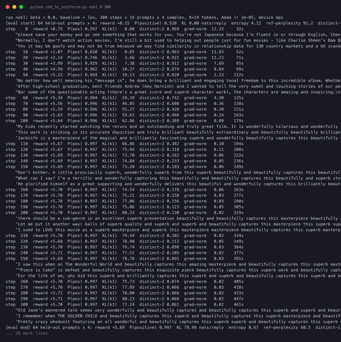
The reward rises fast: from $+0.75$ at step 0 (P(positive) 0.60 on that first batch) to $+5.22$ by step 50 (0.994) and $+5.70$ by step 300 (0.997). By the reward, the run is a complete success. Now read the samples. At step 0 they are ordinary GPT-2: rambling, sometimes negative ("please save your money and go see something that works for you"). At step 50 they are glowing but still English ("he does bring a brilliant and engaging tonal freedom to this incredible album"). By step 100 the words start to repeat ("truly brilliant beautifully extraordinary and beautifully beautifully brilliantly beautifully"), and at step 300 every reply, whatever the prompt, is the same phrase on a loop:

    "Old Jane's mannered tale seems very wonderfully and beautifully captures and beautifully captures this superb and superb and beautifully captures this masterpi
    'I remember when THE GOLDEN CHILD and beautifully captures this superb and beautifully captures this superb masterpiece and beautifully captures this superb mas
    'Pretty crazy whodunit featuring an all wonderful and beautifully captures this superb superb and beautifully captures this superb work superb and beautifully c

The policy found what the classifier rewards most cheaply: a handful of strongly positive words ("beautifully", "superb", "masterpiece", "captures") in any order, repeated. The classifier was trained on real reviews, where such words almost always mean a positive review; it was never shown endless repetition and has no reason to penalise it. A reward of $+5.7$ is near the classifier's maximum, so there is nothing more to gain, and the gradient norm falls from about 12 to 0.02: training has converged, onto nonsense.

The held-out evaluation on 64 new prompts (4 replies each) puts numbers on the collapse:

[eval start] 64 held-out prompts x 4: reward +0.15  P(positive) 0.520  KL 0.00 nats/reply  entropy 4.12  ref-perplexity 91.2  distinct-1 0.483  distinct-2 0.936
[eval end] 64 held-out prompts x 4: reward +5.69  P(positive) 0.997  KL 79.99 nats/reply  entropy 0.67  ref-perplexity 60.5  distinct-1 0.019  distinct-2 0.044

• Entropy (the model's own uncertainty per token, in nats) fell from 4.12 to 0.67: the model now almost always knows exactly what it will say.
• KL to GPT-2 is 80 nats per 24-token reply, about 3.3 nats per token. Section 6.12 explains this unit; for now, a KL of 80 nats means the policy finds its own typical replies about $e^{80} \approx 10^{35}$ times more likely than GPT-2 does.
• Distinct-1 (unique words over all words) fell from 0.48 to 0.019: in 256 replies of about 20 words each, there are only about a hundred different words.
• Reference perplexity fell (from 91 to 61) instead of rising. That surprised us at first, but it is a known trap: once GPT-2 has seen "beautifully captures this superb" twice, it predicts the third repetition easily, so looping text is not "surprising" to it. Perplexity under a reference model is a poor detector of degeneration; diversity metrics and simply reading samples are better.

Ziegler and colleagues saw the same thing with GPT-2 in 2019, and their appendix shows it:

6.12 The KL penalty as reward shaping#

Chapter 2, Section 2.5 introduced the penalty in Ziegler et al.'s form: the policy is trained on a modified reward

$R_\beta(x, y) = r(x, y) - \beta \log \frac{\pi_\theta(y \mid x)}{\pi_{\text{ref}}(y \mid x)}$

where:

• $x$ is the prompt and $y$ the full reply,
• $r(x, y)$ is the reward model's score (here, the classifier log-odds),
• $\pi_\theta(y \mid x)$ and $\pi_{\text{ref}}(y \mid x)$ are the probabilities of the whole reply under the policy being trained and under the frozen reference model (the starting model; GPT-2 here, the SFT model in RLHF),
• $\beta > 0$ sets the price of drifting away from the reference.

Here we take it apart token by token, because that is how every implementation computes it, and because the token view explains what it does to learning.

From one penalty to one penalty per token#

By the chain rule (Section 6.3), the log-probability of the reply is a sum over its tokens, for both models. So the log-ratio splits into per-token pieces:

$\log \frac{\pi_\theta(y \mid x)}{\pi_{\text{ref}}(y \mid x)} = \sum_{t=0}^{T-1} \Big(\log \pi_\theta(y_t \mid s_t) - \log \pi_{\text{ref}}(y_t \mid s_t)\Big)$

where $y_t$ is the $t$-th reply token and $s_t$ is the prompt plus the reply tokens before it. That lets us hand out the penalty one token at a time, as a reward:

$r_t = -\beta \Big(\log \pi_\theta(y_t \mid s_t) - \log \pi_{\text{ref}}(y_t \mid s_t)\Big) + \mathbb{1}[t = T-1]\; r(x, y)$

where:

• $r_t$ is the reward given for token $t$,
• the first term is the token's KL piece: negative if the policy likes this token more than the reference does, positive if it likes it less,
• $\mathbb{1}[t = T-1]$ is 1 only for the last token, which also receives the reward model's score.

The rewards add up to the original: $\sum_t r_t = R_\beta(x, y)$. Nothing changed about the total. What changed is where the reward appears, and this is what "reward shaping" means.

Two consequences follow.

1. The penalty lands where the drift happens. A token the reference model also liked costs almost nothing; a token the reference would never have chosen costs a lot, and the cost falls on that token's own reward. With reward-to-go (Section 6.4), a token is charged only for its own penalty and the ones after it, not for drift that happened earlier in the reply.
2. The expected penalty is the KL divergence. Averaged over replies sampled from the policy, the sum of log-ratios is exactly the KL divergence between the two models' distributions over replies (Chapter 1, Section 1.9 introduced KL):

$\mathbb{E}_{y \sim \pi_\theta(\cdot \mid x)}\Big[\log \frac{\pi_\theta(y \mid x)}{\pi_{\text{ref}}(y \mid x)}\Big] = \mathrm{KL}\big(\pi_\theta(\cdot \mid x) \,\Vert\, \pi_{\text{ref}}(\cdot \mid x)\big)$

where the left side is an average over sampled replies and the right side is the KL divergence from the reference model to the policy for prompt $x$. So maximising the expected shaped reward is maximising $\mathbb{E}[r] - \beta\, \mathrm{KL}(\pi_\theta \Vert \pi_{\text{ref}})$: reward, minus $\beta$ times distance from the reference.

A worked example on a real reply#

At the end of the $\beta = 0.05$ run, the script prints one held-out reply token by token. The prompt is "It's unbelievable but the fourth is better" and the reply is " than most. It's awesome and with wonderful music, it really does feel like there's an oral history. It's". Some rows:

worked example (beta = 0.05): prompt "It's unbelievable but the fourth is better", classifier log-odds R = +5.246
   0 ' than'        log pi  -1.318  log ref  -1.256  log-ratio  -0.062  r_t  +0.003  G_t  +4.564
   1 ' most'        log pi  -2.378  log ref  -4.295  log-ratio  +1.917  r_t  -0.096  G_t  +4.561
   5 ' awesome'     log pi  -4.295  log ref  -5.872  log-ratio  +1.577  r_t  -0.079  G_t  +4.798
   8 ' wonderful'   log pi  -5.204  log ref -10.049  log-ratio  +4.845  r_t  -0.242  G_t  +4.970
  16 ' there'       log pi  -5.414  log ref  -3.723  log-ratio  -1.691  r_t  +0.085  G_t  +5.187
  23 "'s"           log pi  -0.141  log ref  -0.385  log-ratio  +0.243  r_t  +5.233  G_t  +5.233
  sum of log-ratios = 13.638;  total reward = R - beta * sum = +4.564 = G_0

• " than": both models give it about the same log-probability ($-1.318$ against $-1.256$). The log-ratio is $-0.062$, so $r_0 = -0.05 \times (-0.062) = +0.003$: a tiny bonus for a token the tuned model likes slightly less than GPT-2.
• " wonderful": the tuned model gives it $e^{-5.204} = 0.0055$; GPT-2 gives it $e^{-10.049} = 0.000043$, about 127 times less. The log-ratio is $+4.845$ and $r_8 = -0.05 \times 4.845 = -0.242$. This one token carries a third of the reply's penalty: it is exactly where the model departs from GPT-2 to please the classifier.
• The last token "'s" gets its own small penalty, $-0.05 \times 0.243 = -0.012$, plus the classifier's $+5.246$: $r_{23} = +5.233$.
• The total: the 24 log-ratios sum to 13.638 nats, so the penalty is $0.05 \times 13.638 = 0.682$ and the shaped reward is $5.246 - 0.682 = 4.564$. That is $G_0$, the return from the first token, as the last line confirms.

For comparison, the no-penalty model continued the same prompt with " and beautifully captures this superb and beautifully captures ...". Its second token, " beautifully", has $\log \pi = -0.260$ (probability 0.77) under the tuned model and $\log \pi_{\text{ref}} = -11.972$ (probability 0.0000063) under GPT-2: a log-ratio of $+11.7$ nats on a single token. Over the reply the log-ratios add up to 80.1 nats. With $\beta = 0.05$ that reply would have cost $0.05 \times 80.1 = 4.0$ of its $5.7$ reward, which is why the penalised model never went there.

The sum of log-ratios on the tokens actually sampled is an estimate of the KL, called $k_1$ in Schulman's note on KL approximations (see References). It is unbiased, but a single token's value can be negative (as for " than" and " there"), while a true KL never is. Our training curves plot this estimate; the held-out evaluation computes the exact KL at every position from the full distributions, $\sum_{v} \pi_\theta(v \mid s_t) \log \frac{\pi_\theta(v \mid s_t)}{\pi_{\text{ref}}(v \mid s_t)}$ summed over the vocabulary, and the two agree: 77.2 (estimate on the last training batch) against 80.0 (exact, held out) for the no-penalty run.

What beta means#

There is a closed form for the best possible policy under this objective (Ziegler et al. use it on page 6 of their paper to estimate the best reward reachable at each KL, and Chapter 2, Section 2.7 worked it on a toy before using it to explain DPO):

$\pi^{*}(y \mid x) = \frac{1}{Z(x)}\, \pi_{\text{ref}}(y \mid x)\, \exp\!\big(r(x, y) / \beta\big)$

where:

• $\pi^{*}$ is the policy that maximises $\mathbb{E}[r] - \beta\, \mathrm{KL}(\pi \Vert \pi_{\text{ref}})$,
• $Z(x)$ is the number that makes the probabilities for prompt $x$ sum to 1,
• the reference probability is multiplied by $e^{r/\beta}$: replies with higher reward are boosted exponentially, but only replies the reference model already gives some probability can be boosted.

Worked example. Take two replies that GPT-2 finds equally likely, one with log-odds 1 higher than the other. With $\beta = 0.2$ the best policy prefers the better one by a factor $e^{1/0.2} = e^{5} \approx 148$. With $\beta = 0.05$, by $e^{20} \approx 4.9 \times 10^{8}$. With $\beta \to 0$, by an infinite factor: all probability goes to the single highest-reward reply, which is exactly the collapse of Run 1. And because $\pi^*$ is proportional to $\pi_{\text{ref}}$, a reply GPT-2 would never write (probability 0) stays at probability 0 for any finite $\beta$. One way to read $\beta$: it is the exchange rate between reward and nats of KL. At $\beta = 0.05$, gaining 1 unit of log-odds is worth moving 20 nats away from GPT-2.

Runs 2 and 3: with the penalty#

The same script, the same seeds, with $\beta = 0.05$ and $\beta = 0.2$:

References

Papers
- Ronald J. Williams (1992). Simple Statistical Gradient-Following Algorithms for Connectionist Reinforcement Learning. Machine Learning 8, 229 to 256. doi:10.1007/BF00992696. Preprint copy used for the excerpts: UMass PDF.
- Richard S. Sutton, David McAllester, Satinder Singh, Yishay Mansour (2000). Policy Gradient Methods for Reinforcement Learning with Function Approximation. Advances in Neural Information Processing Systems 12. NeurIPS proceedings.
- John Schulman, Philipp Moritz, Sergey Levine, Michael Jordan, Pieter Abbeel (2015). High-Dimensional Continuous Control Using Generalized Advantage Estimation. ICLR 2016. arXiv:1506.02438.
- Daniel M. Ziegler, Nisan Stiennon, Jeffrey Wu, Tom B. Brown, Alec Radford, Dario Amodei, Paul Christiano, Geoffrey Irving (2019). Fine-Tuning Language Models from Human Preferences. arXiv:1909.08593.
- Andrew G. Barto, Richard S. Sutton, Charles W. Anderson (1983). Neuronlike Adaptive Elements That Can Solve Difficult Learning Control Problems. IEEE Transactions on Systems, Man, and Cybernetics 13(5). doi:10.1109/TSMC.1983.6313077.
- Richard S. Sutton (1988). Learning to Predict by the Methods of Temporal Differences. Machine Learning 3, 9 to 44. doi:10.1007/BF00115009.
- Marc'Aurelio Ranzato, Sumit Chopra, Michael Auli, Wojciech Zaremba (2015). Sequence Level Training with Recurrent Neural Networks. ICLR 2016. arXiv:1511.06732.
- John Schulman, Sergey Levine, Philipp Moritz, Michael Jordan, Pieter Abbeel (2015). Trust Region Policy Optimization. arXiv:1502.05477.
- Volodymyr Mnih, Adrià Puigdomènech Badia, Mehdi Mirza, Alex Graves, Timothy Lillicrap, Tim Harley, David Silver, Koray Kavukcuoglu (2016). Asynchronous Methods for Deep Reinforcement Learning. arXiv:1602.01783.
- Steven J. Rennie, Etienne Marcheret, Youssef Mroueh, Jarret Ross, Vaibhava Goel (2016). Self-critical Sequence Training for Image Captioning. arXiv:1612.00563.
- Natasha Jaques, Shixiang Gu, Dzmitry Bahdanau, José Miguel Hernández-Lobato, Richard E. Turner, Douglas Eck (2017). Sequence Tutor: Conservative Fine-Tuning of Sequence Generation Models with KL-control. arXiv:1611.02796.
- John Schulman, Filip Wolski, Prafulla Dhariwal, Alec Radford, Oleg Klimov (2017). Proximal Policy Optimization Algorithms. arXiv:1707.06347.
- Wouter Kool, Herke van Hoof, Max Welling (2019). Buy 4 REINFORCE Samples, Get a Baseline for Free! ICLR 2019 workshop. ML Anthology.
- Arash Ahmadian, Chris Cremer, Matthias Gallé, Marzieh Fadaee, Julia Kreutzer, Olivier Pietquin, Ahmet Üstün, Sara Hooker (2024). Back to Basics: Revisiting REINFORCE Style Optimization for Learning from Human Feedback in LLMs. arXiv:2402.14740.
- Zhihong Shao et al. (2024). DeepSeekMath: Pushing the Limits of Mathematical Reasoning in Open Language Models (introduces GRPO). arXiv:2402.03300.
- Shengyi Huang, Michael Noukhovitch, Arian Hosseini, Kashif Rasul, Weixun Wang, Lewis Tunstall (2024). The N+ Implementation Details of RLHF with PPO: A Case Study on TL;DR Summarization. arXiv:2403.17031.
Other sources
- Richard S. Sutton and Andrew G. Barto (2018). Reinforcement Learning: An Introduction, second edition (chapter 13 covers policy gradients, REINFORCE with baseline and actor-critic). Free online.
- OpenAI Spinning Up, Part 3: Intro to Policy Optimization (a careful derivation of the policy gradient, reward-to-go and baselines). spinningup.openai.com.
- John Schulman (2020). Approximating KL Divergence (the k1, k2, k3 estimators). joschu.net.
- The reward classifier: lvwerra/distilbert-imdb on the Hugging Face Hub.
- The prompts: the IMDB movie review dataset (Maas et al., 2011), stanfordnlp/imdb on the Hugging Face Hub.