How Models Are Trained · Part 2 · Base To Instruction Follower

Chapter 5 · Supervised fine-tuning: teaching it to follow instructions

Supervised fine-tuning from the inside: the same loss on different data with the prompt masked out, the history of instruction datasets from FLAN to Tulu 3, chat templates, a worked masked loss on real tokens, hyperparameters and packing, LoRA and QLoRA with their maths, catastrophic forgetting, and a real LoRA fine-tune of Qwen2.5-0.5B on a laptop GPU.

Goal: by the end of this chapter you can explain exactly what changes when a base model is fine-tuned to follow instructions (and what does not), trace where instruction datasets came from, build a training example in a chat template with the right tokens masked, compute the SFT loss by hand on real tokens, choose sensible hyperparameters, and explain LoRA and QLoRA down to the parameter count. You will also run a LoRA fine-tune of Qwen2.5-0.5B on a laptop GPU, compare its answers before and after on the same prompts, measure it on held-out data and on simple instruction-following checks, and measure what it forgot.

5.1 What changes from pretraining#

Chapter 4 ended with a base model that knows a lot but behaves like a document continuer. Asked "The chemical symbol for gold is", it preferred a blank line, because that is what worksheets do. Chapter 1 showed the same model, given a question in a chat template, rambling on without ending its turn. Supervised fine-tuning (SFT) is the step that fixes this.

Three things change, and one does not.

1. The data. Pretraining used trillions of tokens of whatever the web contains. SFT uses thousands to about a million chosen examples, each a prompt with a good response.
2. The format. Each example is written in a chat template, with special tokens that mark who is speaking and where each turn ends (Chapter 1, Section 1.8).
3. What counts in the loss. Only the response tokens are trained on. The prompt is there as context but its tokens are masked: the model is not taught to write user messages.
4. The loss itself does not change. It is still the cross-entropy of the next token, exactly as in Chapter 1 and Chapter 4.

The amount of compute is tiny by comparison. Our hands-on run in Section 5.9 fine-tunes on 114,146 reply tokens; Qwen2.5-0.5B was pretrained on 18 trillion. That is a ratio of about 160 million to one, and yet the behaviour changes completely. This contrast is the key to understanding SFT: it does not teach the model new knowledge so much as it teaches it which of the things it can already do to do now, and in what format. The LIMA paper put this sharply:

"Superficial" is a strong word, and later work has nuanced it: SFT on mathematics or code data does improve those skills, and the large modern SFT mixtures (Section 5.2) are far bigger than 1,000 examples. But as a first approximation it is right, and our own experiment will show it: a short fine-tune changes how the model answers far more than what it knows.

5.2 A short history of instruction data#

Chapter 2 told the overall story from 2017 to 2025, including the "instruction" thread that ran alongside RLHF. Here we look inside the datasets, because their design choices are still the choices you face when you build an SFT set.

5.2.1 Reformatting existing datasets: FLAN, T0, Super-NaturalInstructions#

The first idea was to reuse what already existed. NLP research had produced hundreds of labelled datasets: translation pairs, sentiment labels, question-answer pairs, entailment judgements. Each could be turned into instructions with a few templates.

The templates are worth seeing, because writing several phrasings of the same task is still standard practice:

T0 (Sanh et al., 2021), from the BigScience collaboration, did the same with a crowd-sourced collection of prompts (P3) on an 11B encoder-decoder model and reported zero-shot results that "often" beat models up to 16 times its size:

Super-NaturalInstructions (Wang et al., 2022) scaled the idea to 1,616 tasks across 76 task types, each with an expert-written definition, positive and negative examples, and explanations:

Google later pushed this line to its limit with Flan-T5 / Flan-PaLM (Chung et al., 2022): 1.8K tasks, plus chain-of-thought examples. Fine-tuning on more tasks kept helping, with diminishing returns.

The weakness of all these sets is visible in the examples: they are NLP benchmark tasks (classify, extract, answer from a passage). Real users ask for emails, plans, explanations, code, stories. A model trained only on these sets answers tersely and in the style of benchmark labels.

5.2.2 Human demonstrations: InstructGPT#

OpenAI's InstructGPT (2022) took the opposite approach: collect prompts that real users sent to its API, and pay people to write good responses.

Human demonstrations are expensive and slow, and InstructGPT's were not released. That opened the door to a cheaper idea.

5.2.3 Models write the data: Self-Instruct and Alpaca#

Self-Instruct (Wang et al., 2022) showed that a model can generate its own instruction data from a small seed:

In March 2023, Stanford's Alpaca combined Self-Instruct with a stronger teacher (OpenAI's text-davinci-003) and the newly released LLaMA 7B:

The dark side of Alpaca-style data is that it imitates its teacher, including its mistakes, and teaches a smaller model to sound like a stronger one without its knowledge. Gudibande et al. (2023) called this "the false promise of imitating proprietary LLMs": imitation models matched the style of ChatGPT but not its factual accuracy.

5.2.4 Quality over quantity: LIMA#

LIMA (Zhou et al., 2023) asked how few examples are really needed:

5.2.5 Modern open recipes: Tulu 2 and Tulu 3#

The Allen Institute's Tulu series is the best-documented open recipe for post-training. Tulu 2 (2023) fine-tuned Llama 2 on a mixture of 326,154 examples drawn from many sources (FLAN, human-written chats, synthetic code and science data) and then applied DPO (previewed in Chapter 2). Tulu 3 (2024) went further:

A common way to make synthetic SFT data better than its teacher's average output is rejection sampling: generate several replies per prompt, score them (with a reward model, a test suite for code, or a check of the final answer for mathematics), and keep only the best. Llama 3's post-training repeated this loop over several rounds, each round's best model generating the next round's SFT data.

The lesson of this history fits in one line: what you fine-tune on matters more than how much, and the best sets are diverse, consistent in style, and checked for correctness.

5.3 The data in our hands-on run#

Our run uses Alpaca-cleaned, a community-cleaned version of the 52K Alpaca set in which obviously wrong or broken examples were repaired. ch5_data.py takes a first look:

rows: 51,760; rows with a non-empty input field: 19,157
most common first words of the instruction: generate 4,608, create 3,611, describe 2,953, write 2,787, what 2,369,
    given 2,180, explain 2,032, name 1,964, identify 1,505, find 1,342, rewrite 1,266, list 1,099
reply length (every 50th row, 1036 rows): median 108 tokens, 90th percentile 348, max 584

Each row has an instruction, an optional input (some context to work on, present in 37% of rows) and an output. The instructions are dominated by a few verbs ("generate", "create", "describe", "write"), a known trait of Self-Instruct-style data: generated instructions are less varied than real user requests. Here is how one row becomes a chat. ch5_common.py puts the instruction (and the input, if any) in the user turn and the output in the assistant turn:

def messages(ex):
    user = ex['instruction'] + ('\n\n' + ex['input'] if ex['input'].strip() else '')
    return [{'role': 'system', 'content': SYSTEM}, {'role': 'user', 'content': user}], ex['output']

SYSTEM is "You are a helpful assistant.", the default system prompt of the Qwen2.5 base tokenizer's template. The result for the second row of the dataset:

<|im_start|>system
You are a helpful assistant.<|im_end|>
<|im_start|>user
What are the three primary colors?<|im_end|>
<|im_start|>assistant
The three primary colors are red, blue, and yellow. These colors are called primary because they cannot be created
by mixing other colors and all other colors can be made by combining them in various proportions. In the additive
color system, used for light, the primary colors are red, green, and blue (RGB).<|im_end|>
90 tokens, of which 64 are learned (the reply and <|im_end|>)

From the full set we draw 1,000 training examples and 100 held-out examples at random, keeping only those that fit in 384 tokens. Section 5.9 explains why the run is this small.

5.4 Chat templates and special tokens, for training#

Chapter 1 walked through the Qwen2.5 chat template token by token at inference time. Training adds three practical points.

First, the template at training time must match the template at use time, exactly. The prompt part of every training example is built by the same apply_chat_template call that will build prompts later, with add_generation_prompt=True, which ends the prompt with <|im_start|>assistant and a line break. The model learns that a reply starts right there. If, at use time, a different system prompt, a missing line break or another family's template is used, the model sees a format it was never trained on.

Second, the turn-ending token is part of the reply. The reply is the answer's tokens followed by <|im_end|> (id 151645). That last token is the single most important token in SFT: it is what teaches the model to stop. (Qwen also has <|endoftext|>, id 151643, which ends documents in pretraining; the base tokenizer uses it as the padding token, which is why padding must be masked out of the loss.)

Third, in a multi-turn conversation, every assistant turn is trained on, and every other turn is masked. ch5_template.py builds a two-turn chat and marks which tokens are learned:

5.5 The SFT loss, with label masking#

The SFT loss is the pretraining loss of Chapter 4 with a mask.

$\mathcal{L}_{\text{SFT}} = -\frac{1}{\sum_{t} m_t} \sum_{t=1}^{T-1} m_t \log p_\theta\left(x_{t+1} \mid x_1, \ldots, x_t\right)$

where:

• $x_1, \ldots, x_T$ are the tokens of one example (prompt followed by reply and <|im_end|>),
• $p_\theta(x_{t+1} \mid x_1, \ldots, x_t)$ is the probability the model with weights $\theta$ gives to the true next token,
• $m_t$ is 1 if token $x_{t+1}$ belongs to the reply (including the final <|im_end|>) and 0 if it belongs to the prompt or is padding,
• the sum of $m_t$ in the denominator is the number of reply tokens, so the loss is an average over reply tokens only.

In code the mask is not a separate tensor: the masked positions simply get the label $-100$, which PyTorch's cross_entropy ignores. From ch5_common.py:

def encode(ex, max_len=512):
    msgs, reply = messages(ex)
    text = tok.apply_chat_template(msgs, add_generation_prompt=True, tokenize=False)   # ends with "<|im_start|>assistant\n"
    prompt = tok(text)['input_ids']
    answer = tok(reply)['input_ids'] + [END]
    ids = (prompt + answer)[:max_len]
    labels = ([-100] * len(prompt) + answer)[:max_len]
    return {'input_ids': ids, 'labels': labels}

def sft_loss(model, ids, lab, att, reduction='mean'):
    logits = model(input_ids=ids, attention_mask=att).logits[:, :-1]
    target = lab[:, 1:]
    return F.cross_entropy(logits.reshape(-1, logits.size(-1)).float(), target.reshape(-1),
                           ignore_index=-100, reduction=reduction)

In encode, the prompt is rendered by the chat template as text and tokenized; the reply is tokenized on its own and END (<|im_end|>) is appended. The labels are a copy of the ids with every prompt position replaced by $-100$. In sft_loss, the model returns one row of logits per position; the logits at position $t$ predict token $t+1$, so the logits drop their last position and the labels drop their first (the token shift of Chapter 1). cross_entropy with ignore_index=-100 averages over the remaining positions only, which is exactly $\mathcal{L}_{\text{SFT}}$.

A worked example on real tokens#

ch5_template.py takes one short example, "Name three primary colours." with the reply "The three primary colours are red, blue and yellow.", and computes the loss of the base model at every position.

-- Qwen2.5-0.5B base
   predict 'The'          loss   2.429   p = 0.0881
   predict ' three'       loss   1.409   p = 0.2444
   predict ' primary'     loss   0.012   p = 0.9882
   predict ' colours'     loss   0.048   p = 0.9532
   predict ' are'         loss   0.144   p = 0.8659
   predict ' red'         loss   0.585   p = 0.5569
   predict ','            loss   0.010   p = 0.9896
   predict ' blue'        loss   0.869   p = 0.4194
   predict ' and'         loss   2.167   p = 0.1145
   predict ' yellow'      loss   0.108   p = 0.8978
   predict '.'            loss   0.755   p = 0.4702
   predict '<|im_end|>'   loss  13.119   p = 0.0000
   masked loss (reply tokens only, 12 tokens) = 1.805
   unmasked loss (all 35 predicted tokens)            = 5.670
   masked loss without the final <|im_end|>                 = 0.776

Each line is one term of the sum: the loss at a reply position is $-\ln p$ of the true token. For " primary" the base model gives probability 0.988, so the loss is $-\ln 0.988 = 0.012$: after "Name three primary colours" and "The three", the word "primary" is almost certain. For " and" it is 2.167, because the model expected a comma (an Oxford-comma list: "red, blue, and yellow"). The masked loss is the average of the 12 values: $(2.429 + 1.409 + \ldots + 13.119) / 12 = 1.805$.

Three things in this table explain most of SFT:

1. The base model already knows the answer. Without the last token, its average loss on this reply is 0.776 nats: it would have produced almost exactly this sentence. SFT does not need to teach it that red, blue and yellow are the primary colours.
2. It has no idea the reply should end. The <|im_end|> token gets probability about $2 \times 10^{-6}$ ($e^{-13.1}$), a loss of 13.1 nats, more than all the other tokens together. This one token is why the base model rambles on, and it is the first thing SFT fixes.
3. Masking matters. Without the mask, the loss averages over all 35 predicted positions and comes out at 5.670, dominated by positions the model is not meant to predict: the system prompt, the role names, the user's question. Training on those would teach the model to write user messages, and it would spend most of its gradient on them.

SFT has few knobs, and the defaults in published recipes are a good start. What each one does:

Learning rate. Much smaller than in pretraining for full fine-tuning: around $10^{-5}$ for models of a few billion parameters (Tulu 3 used $5 \times 10^{-6}$ for its 8B model and $2 \times 10^{-6}$ for its 70B model). The pretrained weights are already good; large steps destroy what is there. LoRA uses much larger rates, typically $10^{-4}$ to $3 \times 10^{-4}$, because its small adapter matrices start at zero and have to grow. Our runs use $2 \times 10^{-4}$ for LoRA and $10^{-5}$ for full fine-tuning, with a short warmup (5% of the steps) and a cosine decay to zero.

Epochs. One to three passes over the data is typical (Tulu 2 and Tulu 3 used 2). With very small, very clean sets more epochs can help: LIMA trained for 15 epochs on its 1,000 examples and picked a checkpoint between the 5th and the 10th by reading answers, because the held-out perplexity did not track answer quality. More epochs lower the training loss but raise the risk of memorizing the exact replies; the held-out loss tells you when to stop.

Batch size. Usually 64 to 128 sequences per step for large runs, built with gradient accumulation (several small batches whose gradients are added before one update). Our runs use 8 examples per step, which is small but fine for 1,000 examples.

Maximum length. Examples longer than the limit are cut. A cut example loses its ending, including the <|im_end|> that teaches stopping, so it is better to drop or filter very long examples than to cut them. We keep only examples that fit in 384 tokens.

Loss over prompts or not. The standard choice, used here, is to mask the prompt. Shi et al. (2024) found that also training on the prompt tokens can help when the replies are short and the dataset is small, but masking is the safe default.

Padding and packing#

Examples have different lengths, and a batch is a rectangle. The simple solution is padding: fill each example up to the longest one in the batch with a pad token, and mask the padding out of both the attention and the loss. The cost is compute spent on nothing.

ch5_template.py measures what padding costs on our 1,000 training examples:

Packing matters a lot for large SFT runs (Tulu 3's examples range from a dozen tokens to several thousand). Our run uses plain padding because the run is small and the code stays simpler, and because packing on the Apple GPU would need the block-diagonal attention to avoid cross-talk between examples. One practical detail did matter on this hardware: the padded length is rounded up to a multiple of 128 tokens. The Apple GPU backend prepares its kernels separately for every new tensor shape, and with a different length at every step the first attempt at this run was about ten times slower.

5.7 LoRA: fine-tuning a few million numbers instead of half a billion#

Full fine-tuning updates every weight, and Chapter 4 showed what that costs: about 16 bytes of training state per parameter, so 7.4 GiB for our 0.5B model and over 100 GiB for a 7B one. It also produces a full copy of the model for every fine-tune. LoRA (Hu et al., 2021) avoids both.

The idea rests on an observation: the change a fine-tune makes to a weight matrix seems to have a much simpler structure than the matrix itself. A $d \times d$ change can be described with far fewer than $d^2$ numbers if it has low rank.

In symbols, for one linear layer:

$h = W_0 x + \frac{\alpha}{r} B A x, \qquad B \in \mathbb{R}^{d_{\text{out}} \times r}, \quad A \in \mathbb{R}^{r \times d_{\text{in}}}$

where:

• $x$ is the layer's input (a vector of length $d_{\text{in}}$) and $h$ its output (length $d_{\text{out}}$),
• $W_0$ is the pretrained weight matrix, $d_{\text{out}} \times d_{\text{in}}$, frozen,
• $A$ maps the input down to $r$ numbers and $B$ maps them back up; only $A$ and $B$ are trained,
• $r$ is the rank, much smaller than $d_{\text{in}}$ and $d_{\text{out}}$ (we use 16),
• $\alpha$ is a fixed scaling constant (we use 32, so the scale $\alpha / r$ is 2).

The trainable parameters per adapted matrix are

$N_{\text{LoRA}} = r\,(d_{\text{in}} + d_{\text{out}}) \quad \text{instead of} \quad d_{\text{in}} \times d_{\text{out}}$

Worked example: a rank-1 update (ch5_lora_math.py). With $B = (1, 0.5, -1, 2)^\top$ and $A = (0.2, -0.4, 0, 0.6)$, the product $BA$ is a full $4 \times 4$ matrix whose first row is $1 \times A = (0.2, -0.4, 0, 0.6)$, second row $0.5 \times A$, and so on: 16 numbers built from 8.

Worked example: Qwen2.5-0.5B. The model has 24 layers, each with 7 linear layers. Their real shapes (ch5_lora_math.py):

  q_proj    W:   896 x   896 =    802,816 weights;  LoRA r=16 adds r(d_in + d_out) = 16 x 1,792 = 28,672
  k_proj    W:   128 x   896 =    114,688 weights;  LoRA r=16 adds r(d_in + d_out) = 16 x 1,024 = 16,384
  v_proj    W:   128 x   896 =    114,688 weights;  LoRA r=16 adds r(d_in + d_out) = 16 x 1,024 = 16,384
  o_proj    W:   896 x   896 =    802,816 weights;  LoRA r=16 adds r(d_in + d_out) = 16 x 1,792 = 28,672
  gate_proj W:  4864 x   896 =  4,358,144 weights;  LoRA r=16 adds r(d_in + d_out) = 16 x 5,760 = 92,160
  up_proj   W:  4864 x   896 =  4,358,144 weights;  LoRA r=16 adds r(d_in + d_out) = 16 x 5,760 = 92,160
  down_proj W:   896 x  4864 =  4,358,144 weights;  LoRA r=16 adds r(d_in + d_out) = 16 x 5,760 = 92,160

(The key and value projections are only 128 wide because Qwen2.5-0.5B uses grouped-query attention: 14 query heads share 2 key-value heads of 64 numbers each.) One layer gets $28{,}672 \times 2 + 16{,}384 \times 2 + 92{,}160 \times 3 = 366{,}592$ LoRA parameters, and 24 layers give $8{,}798{,}208$: 1.78% of the model's 494,032,768. The peft library reports exactly the same number.

Three properties make LoRA practical:

1. It starts as a no-op. Because $B = 0$ at the start, $BAx = 0$ and the model behaves exactly like the base model. ch5_lora_math.py checks this: the largest difference between the logits with and without the adapter is $0.0$.
2. It can be merged. After training, $W' = W_0 + \frac{\alpha}{r} BA$ is an ordinary matrix of the original shape. The merged model runs at the original speed. Or the adapters can be kept separate and swapped: one base model, many small task adapters of a few megabytes each.
3. It needs far less memory. Gradients and optimizer state exist only for the adapter parameters.

Which matrices to adapt, and which rank? The original paper adapted only the attention query and value matrices of GPT-3 and found that a rank as small as 1 to 8 was often enough there. Later practice (QLoRA, and "LoRA learns less and forgets less") found that adapting all linear layers, including the MLP, matters more than the rank; we follow that. The rank is a trade-off covered in Section 5.10: higher ranks learn more and forget more.

5.8 QLoRA, briefly#

LoRA freezes the base weights but still stores them in 16 bits. For a 65B model that is 121 GiB, more than any single GPU holds. QLoRA (Dettmers et al., 2023) stores the frozen weights in 4 bits:

We do not use QLoRA in the hands-on run: the 4-bit kernels it relies on (the bitsandbytes library) target NVIDIA GPUs, and a 0.5B model fits in a laptop's memory anyway. For a 7B model or larger on a single consumer GPU, it is the standard choice.

5.9 Hands-on: LoRA fine-tuning of Qwen2.5-0.5B on a laptop#

Time to change some weights. The plan:

• Model: Qwen/Qwen2.5-0.5B, the base model of Chapters 1 and 4.
• Data: 1,000 random Alpaca-cleaned examples for training, 100 others held out (Section 5.3).
• Method: LoRA with rank 16 and $\alpha = 32$ on all seven linear layers of every block, learning rate $2 \times 10^{-4}$, 8 examples per step, one epoch (125 steps), warmup over the first 6 steps and cosine decay to zero.
• Evaluation: the held-out loss before, during and after; twelve instruction-following checks; answers to the same prompts before and after; and two probes of forgetting (Section 5.10). The same evaluation runs on the base model and on Qwen's own Qwen2.5-0.5B-Instruct, as references.

The training script#

Here is the core of ch5_sft.py, slightly simplified:

train, val = load_split()                                   # 1,000 + 100 encoded examples
model = load('Qwen/Qwen2.5-0.5B')                           # fp32 weights on the Apple GPU
cfg = LoraConfig(r=16, lora_alpha=32, lora_dropout=0.05, task_type='CAUSAL_LM',
                 target_modules=['q_proj', 'k_proj', 'v_proj', 'o_proj', 'gate_proj', 'up_proj', 'down_proj'],
                 trainable_token_indices={'embed_tokens': [151644, 151645]})   # see "The first run" below
model = get_peft_model(model, cfg)
params = [p for p in model.parameters() if p.requires_grad]
opt = torch.optim.AdamW(params, lr=2e-4, weight_decay=0.0)

steps = len(train) // 8                                     # one epoch: 125 steps
for step in range(steps):
    lr = lr_at(step, 2e-4, max(1, steps // 20), steps, floor=0.0)
    for g in opt.param_groups:
        g['lr'] = lr
    ids, lab, att = (t.to('mps') for t in collate([train[i][1] for i in order[step * 8:(step + 1) * 8]]))
    with torch.autocast('mps', dtype=torch.bfloat16):
        loss = sft_loss(model, ids, lab, att)
    loss.backward()
    torch.nn.utils.clip_grad_norm_(params, 1.0)
    opt.step()
    opt.zero_grad(set_to_none=True)

Block by block:

• Data and model. load_split draws and encodes the examples with the masked labels of Section 5.5. The base model is loaded in fp32; the matrix multiplications will run in bf16 under autocast, the mixed precision of Chapter 4.
• LoRA. LoraConfig describes the adapters: rank 16, scale $\alpha = 32$, dropout 0.05 on the adapter's input (a mild regularizer), and the seven layer names to adapt. get_peft_model freezes every original weight and inserts an $A$ and a $B$ beside each of the $7 \times 24 = 168$ chosen matrices. The trainable_token_indices line also makes two rows of the embedding trainable; the next subsection explains why it is there.
• Optimizer. Only parameters with requires_grad (the adapters) go to AdamW, so optimizer state exists only for them. No weight decay, a common choice for LoRA.
• The loop. The same schedule function as Chapter 4 (lr_at), now with warmup over 5% of the steps and decay to 0. collate pads 8 examples to a common length (rounded up to a multiple of 128) and returns the ids, the labels with $-100$ on prompt and padding, and the attention mask. sft_loss is the masked loss of Section 5.5. Gradient clipping at 1.0 and the AdamW step finish the iteration.

After training, the same script runs the twelve checks, the forgetting probes and three open prompts, and saves the adapter (35 MB).

The first run: a model that could not say "stop"#

The first run used plain LoRA, without the trainable_token_indices line. Its loss went down nicely (held-out loss from 1.532 to 1.386), its answers took on the Alpaca style, and yet it failed most of the checks in a strange way. Here is where it should have ended its turn, as ch5_sft.py lora_plain logged it:

'1. Apple\n2. Banana\n3. Orange.:UIControl\n1. Apple\n2. Banana\n3'
'The sky on a clear day is blue.看查看'
'HELLO. заявк\n_QUOTES\nYou are a helpful assistant._QUOTES\n_QU'
'The sum of 12 and 30 is 42. The answer is 42.<quote>'
'Bonjour. אהבתי\nThe translation of "good morning" into French'

Each answer is right and correctly shaped, and then, exactly where <|im_end|> should come, the model emits a random-looking token from some other language or from code, and carries on. The model clearly learned when to stop. It could not learn how, and the reason is in the embedding matrix.

Qwen2.5-0.5B ties its input embedding and its output layer: one $151{,}936 \times 896$ matrix is used both to turn token ids into vectors and to turn the final hidden vector into a score per token. LoRA, as configured, freezes it. ch5_special_tokens.py looks at the row of <|im_end|>:

mean row norm over the 151,643 ordinary tokens: 0.464
  <|endoftext|>   id 151643: norm 0.599
  <|im_start|>    id 151644: norm 0.301
  <|im_end|>      id 151645: norm 0.301
rows almost identical to <|im_end|> (cosine > 0.9999 and every number within 0.001): 2256 (including itself)
   e.g. id 124 '�': cosine 1.000000, largest difference in any of the 896 numbers 1.22e-04
if they tied exactly, p(<|im_end|>) could not exceed 1/2256, a loss of at least ln(2256) = 7.72 nats

The <|im_end|> row is one of 2,256 rows that hold the same numbers, to within bf16 rounding: rows of tokens that were (almost) never seen in pretraining, such as rare byte fragments, unused reserved ids and <|im_start|>/<|im_end|> themselves. Their vectors never moved far from a common starting point. In the output layer, the score of a token is the dot product of the hidden vector with that token's row, so whatever hidden vector the model produces, those 2,256 tokens get practically the same score. The model could push its hidden state towards "this group", which is exactly what it learned to do at the end of an answer, but it had no way to prefer <|im_end|> over its 2,255 twins. Greedy decoding then picks whichever twin has a tiny rounding edge: 看查看, .:UIControl, <quote>. On the worked example of Section 5.5, the plain-LoRA loss on <|im_end|> was 8.44 nats, just above the 7.72 floor that a perfect tie would impose.

The fix is small: make the two rows of <|im_start|> and <|im_end|> trainable. That is 1,792 extra numbers (2 rows of 896); peft keeps them as a separate "delta" so the rest of the matrix stays frozen. With it, the loss on <|im_end|> in the worked example drops to 0.004.

Results#

With the two rows trainable, the second run took 27 minutes. Its full log:

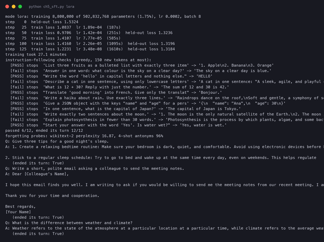
The loss curves of both runs:

held-out loss per reply token (100 Alpaca examples never seen in training)
  Qwen2.5-0.5B base                1.532
  plain LoRA, after 125 steps      1.386
  LoRA + token rows, after 125     1.318
  full fine-tuning, after 125      1.375
  Qwen2.5-0.5B-Instruct            1.328

Most of the drop happens in the first 50 steps (1.532 to 1.324). The difference between the two LoRA runs, about 0.07, is almost all one token: the <|im_end|> at the end of each reply, which costs the plain run about 8 nats and the fixed run almost nothing. Our model ends slightly below Qwen's own Instruct model on this held-out set, which says more about the test than about the models: the held-out examples are Alpaca-style, exactly like our training data, while Qwen's post-training aimed at a much broader target. A held-out loss measures how well a model imitates this distribution, not how good an assistant it is.

For comparison, ch5_sft.py full fine-tuned all 494,032,768 weights on the same data, in the same order, at a learning rate of $10^{-5}$ (with 7.4 GiB of training state instead of about 1 GiB). It took 10 minutes, ended at a held-out loss of 1.375, and, without any special treatment, learned to end its turn: full fine-tuning updates the embedding matrix, including the <|im_end|> row. Its held-out loss is higher than the LoRA run's, which says more about our choice of learning rates than about the methods: $10^{-5}$ for 125 small steps is cautious, while $2 \times 10^{-4}$ on LoRA's zero-initialized adapters moves faster. A sweep of learning rates would be needed to compare the two methods fairly, and it is the first thing to try if you repeat this experiment.

The answers tell more. The same prompt, before and after:

Both models know the material; the base model already lists sensible tips. The difference is the shape: a numbered list of exactly three tips, each with a short explanation, and then <|im_end|>. The answers to "What is the difference between weather and climate?" show a smaller effect on content:

base:      "Weather refers to the average temperature and weather conditions of a particular location over a period
            of time. Climate, on the other hand, refers to the average weather conditions ..."
LoRA SFT:  "Weather refers to the state of the atmosphere at a particular location at a particular time, while climate
            refers to the average weather conditions over a long period of time. ..."
Instruct:  "Weather refers to the average conditions of an area over time, such as temperature, precipitation, ..."

The base model's definition of weather is muddled (weather is not an average); the fine-tuned model states the textbook distinction in its first sentence; Qwen's Instruct model, interestingly, repeats the base model's mistake. One prompt proves nothing, but it is a reminder that SFT data also nudges which of the things a model half-knows it says first. None of the evaluation prompts appears in our 1,000 training examples; the closest is one training instruction on a related topic, "Explain why a good night's sleep is important."

And the twelve checks, run greedily with at most 150 new tokens. A check passes only if the model ends its turn by itself and meets the constraint (exactly three bullet points, one word, only "HELLO", and so on):

                     passed   ended its turn
base model            4/12        6/12
plain LoRA            2/12        6/12
LoRA + token rows     6/12       12/12
full fine-tuning      6/12       12/12
Qwen2.5-0.5B-Instruct 9/12       12/12

Read the rows from the bottom up. Qwen's Instruct model, trained with a large SFT set and then preference tuning, passes 9 of 12 and always ends its turn. Our LoRA model ends its turn every time (from 6 of 12 for the base model) and doubles the base model's passes from 4 to 6, after 125 steps on 1,000 Alpaca examples. Its failures are instructive: asked to answer "in one word", it writes the full sentence "The sky on a clear day is blue."; asked for "just the number", it writes "The sum of 12 and 30 is 42."; asked for "exactly two sentences", it writes a numbered list. Alpaca's replies are full, polite sentences, almost never one-word answers or exact counts, so the model learned that style and nothing about precise constraints. SFT teaches what is in the data. Tulu 3 added a whole synthetic dataset of precise instruction-following examples ("Tulu 3 Persona IF" in its SFT mix) for exactly this reason.

Two smaller observations. The base model's 4 passes are not nothing: Qwen2.5's pretraining data clearly contains instruction-like text, and the base model often answers sensibly before it rambles on. And the plain LoRA run scored lower than the base model, 2 of 12, because its answers were better shaped but almost never ended cleanly. A single broken token can cost more than everything else gains.

5.10 Catastrophic forgetting#

Fine-tuning moves weights that pretraining set. Some of what those weights did may be lost.

Luo et al. (2023) measured it during continual instruction tuning of models from 1B to 7B parameters and found that general knowledge, reasoning and reading comprehension all degraded as fine-tuning went on, and, surprisingly, that within their range larger models forgot more. Biderman et al. (2024) compared LoRA with full fine-tuning on code and mathematics and summarized the result in their title, "LoRA learns less and forgets less":

Our runs are far too short to show much forgetting, but we can measure it with two cheap probes of what the base model could already do, run in exactly the same way on every model (ch5_common.py):

• Perplexity on Wikipedia text (the first 20,480 tokens of the wikitext-2 test set, no chat template): a probe of plain language modelling, the thing pretraining optimized.
• 4-shot antonyms in a plain-text prompt: Chapter 4's in-context learning task, 26 test words.

                        wikitext-2 perplexity   4-shot antonyms
base model                     16.65                 96%
plain LoRA                     16.86                 96%
LoRA + token rows              16.87                 96%
full fine-tuning               16.90                 92%
Qwen2.5-0.5B-Instruct          18.33                 92%

Our LoRA runs raised the Wikipedia perplexity by about 1.3% (16.65 to 16.87) and did not change the antonym score: almost nothing was forgotten, as expected from 125 small steps on 1.8% of the parameters. Full fine-tuning of all 494M weights for the same 125 steps (at a learning rate of $10^{-5}$) ended in practically the same place: perplexity 16.90, and one antonym fewer (92%, that is 24 of 26 words instead of 25), a difference too small to call. Qwen's Instruct model, after a much longer post-training, is 10% worse than its base model at predicting Wikipedia text (18.33 against 16.65) and slightly worse at the plain-text few-shot task. That is the price of turning a document continuer into an assistant: some of its raw language-modelling sharpness goes, in exchange for the behaviour of Section 5.9.

What reduces forgetting in practice:

• Use LoRA, or a lower learning rate and fewer epochs for full fine-tuning.
• Mix in general data. Adding some pretraining-style text or general instruction data to a narrow fine-tuning set keeps old abilities in use. Tulu 3's broad SFT mix is partly this.
• Measure it. Keep a few probes of what the base model could do (perplexity on general text, a few-shot task, a knowledge benchmark) and run them before and after, as we did here.

5.11 A checklist for SFT#

Most failed fine-tunes fail for boring reasons. Before reading anything into a result, check these, in this order:

1. The template. Print one fully rendered training example and one rendered inference prompt, and compare them character by character. The training prompt must end exactly where the inference prompt ends (the generation prompt).
2. The mask. Print the labels next to the tokens, as ch5_template.py does. Only reply tokens and the closing turn token should be learned; padding and prompt must be $-100$.
3. The end token. Make sure every reply ends with the turn-ending token, that truncation never cuts it off, and that it can be learned: if the embeddings are frozen, check whether its row is a trained row (Section 5.9).
4. The data. Look at 50 random examples by eye. Remove duplicates and near-duplicates (the MinHash of Chapter 4 works here too), remove examples that overlap with your test sets, and check that the style is consistent: the model will copy whatever style dominates.
5. The learning rate. About $10^{-5}$ for full fine-tuning of small models (lower for big ones), about $10^{-4}$ to $3 \times 10^{-4}$ for LoRA. If the training loss jumps up in the first steps, it is too high.
6. The evaluation. Measure three things, not one: a held-out loss on data like the training data; behaviour on prompts unlike it (checks with verifiable constraints, or a benchmark); and a few probes of what the base model could already do, to catch forgetting.

5.12 Where SFT stops#

SFT is powerful because it is simple: show the model what a good reply looks like and train it to imitate. That simplicity is also its limit.

• It can only imitate. The model learns to produce replies like the ones in the data. If the data has errors, the model learns the errors; Qwen's own Instruct model told us, in the "two sentences about the moon" check, that the moon is "384,400 kilometers in diameter" (that is its distance from Earth). SFT gives no signal about which of two plausible replies is better.
• It cannot say "not like this". Every training example is a positive example. There is no way to show the model a bad reply and push it away from it, which matters for safety and for subtle qualities like honesty or conciseness.
• It learns a style, including its weaknesses. Our model learned Alpaca's full-sentence style so well that it would not answer in one word when asked to.
• It trains on the teacher's text, not on the model's own. At use time the model continues its own words, mistakes included, which it never saw in training.

Preference-based training addresses exactly these limits. A reward model is trained from human comparisons between two replies, so that "better" becomes a number; RLHF with PPO, DPO and GRPO, which Chapter 2 previewed, then use that signal to move the model towards better replies and away from worse ones. They almost always start from an SFT model like the one we just built.

References#

Papers#

• Wei, J. et al. (2021). Finetuned Language Models Are Zero-Shot Learners (FLAN). arXiv:2109.01652
• Sanh, V. et al. (2021). Multitask Prompted Training Enables Zero-Shot Task Generalization (T0). arXiv:2110.08207
• Wang, Y. et al. (2022). Super-NaturalInstructions: Generalization via Declarative Instructions on 1600+ NLP Tasks. arXiv:2204.07705
• Chung, H. W. et al. (2022). Scaling Instruction-Finetuned Language Models (Flan-T5, Flan-PaLM). arXiv:2210.11416
• Ouyang, L. et al. (2022). Training language models to follow instructions with human feedback (InstructGPT). arXiv:2203.02155
• Wang, Y. et al. (2022). Self-Instruct: Aligning Language Models with Self-Generated Instructions. arXiv:2212.10560
• Gudibande, A. et al. (2023). The False Promise of Imitating Proprietary LLMs. arXiv:2305.15717
• Zhou, C. et al. (2023). LIMA: Less Is More for Alignment. arXiv:2305.11206
• Ivison, H. et al. (2023). Camels in a Changing Climate: Enhancing LM Adaptation with Tulu 2. arXiv:2311.10702
• Lambert, N. et al. (2024). Tulu 3: Pushing Frontiers in Open Language Model Post-Training. arXiv:2411.15124
• Shi, Z. et al. (2024). Instruction Tuning With Loss Over Instructions. arXiv:2405.14394
• Hu, E. J. et al. (2021). LoRA: Low-Rank Adaptation of Large Language Models. arXiv:2106.09685
• Dettmers, T. et al. (2023). QLoRA: Efficient Finetuning of Quantized LLMs. arXiv:2305.14314
• Zhou, J. et al. (2023). Instruction-Following Evaluation for Large Language Models (IFEval). arXiv:2311.07911
• Biderman, D. et al. (2024). LoRA Learns Less and Forgets Less. arXiv:2405.09673
• Luo, Y. et al. (2023). An Empirical Study of Catastrophic Forgetting in Large Language Models During Continual Fine-tuning. arXiv:2308.08747
• Qwen Team (2024). Qwen2.5 Technical Report. arXiv:2412.15115

Other sources#

• Taori, R. et al. (2023). Alpaca: A Strong, Replicable Instruction-Following Model. Stanford CRFM blog. crfm.stanford.edu/2023/03/13/alpaca.html
• The Alpaca-cleaned dataset used in the hands-on run. huggingface.co/datasets/yahma/alpaca-cleaned
• The base and instruct models: Qwen/Qwen2.5-0.5B and Qwen/Qwen2.5-0.5B-Instruct.
• The peft library used for LoRA. huggingface.co/docs/peft
• The scripts behind every number in this chapter: code/training/ch5_*.py, with their saved output in code/training/results/.