How Models Are Trained · Part 2 · Base To Instruction Follower

Chapter 4 · Pretraining: learning from the whole internet

Pretraining from the inside: how web text is collected, filtered and deduplicated, how it is tokenized, what training costs (C = 6ND), what scaling laws say about model size and data, the learning-rate schedule, batch size and mixed precision, and a real 12M-parameter GPT pretrained on a laptop GPU.

Goal: by the end of this chapter you can explain every stage that turns raw web pages into a base model: how the text is collected, cleaned, deduplicated and scored; how it is cut into tokens; how much compute a run needs and how to calculate it; how scaling laws decide the size of the model and the amount of data; why the learning rate rises and then falls, why batches are large, and why training runs in 16-bit numbers. You will also pretrain a small GPT yourself on a laptop GPU, watch its loss fall and its stories improve, and then probe a real base model to see what pretraining alone puts inside it.

4.1 What pretraining is#

Chapter 1 described a language model as a machine that reads some tokens and gives a probability to every possible next token. It showed the loss used to train it (cross-entropy), how that loss turns into perplexity, and a tiny training loop. It also drew the whole pipeline, from a base model to an assistant. This chapter zooms into the first and by far the most expensive box of that pipeline: pretraining.

The objective is the same next-token cross-entropy you met in Chapter 1. What makes pretraining a field of its own is everything around that objective, and the scale at which it runs. A modern run has to answer questions like these:

• Where do ten trillion tokens of text come from, and how do you remove the spam, the duplicates and the junk?
• How is text cut into tokens?
• How large should the model be, and how many tokens should it see, for a given budget of compute?
• How fast should it learn at each moment, how many examples should be in each step, and with how many bits per number?
• What does the model actually know when it is done?

We will take these in order. Every number in this chapter comes either from a paper (shown in a PAPER box, with the excerpt) or from a script in code/training/ that you can run yourself. The hands-on run in Section 4.11 pretrains a 12-million-parameter GPT on 12 million tokens in about eight minutes on a laptop's Apple GPU. It is a toy, tens of billions of times smaller in compute than a frontier model, but it has every piece a real run has.

4.2 The data: where trillions of words come from#

4.2.1 Common Crawl: a copy of the public web#

Almost every large pretraining corpus starts from Common Crawl, a nonprofit that has crawled the public web since 2008 and gives the results away. Each crawl ("snapshot") holds a few billion pages and is published in three file formats.

To see what this raw material looks like, the script ch4_data.py downloads the first 12 MB of one WET file of the August 2024 crawl and reads every page in it. The first numbers are a good reality check:

raw documents: 3,964   characters: 23,632,096
top languages (Common Crawl header, CLD2): eng 1405, zho 727, rus 296, jpn 246, deu 152, fra 148, spa 144, pol 94

Only 35% of the pages are English. Here are the first few English pages the filters threw away, as the script recorded them (the text is collapsed to one line):

word count       | http://16beavergroup.org/articles/...     | One moment, please... Please wait while your request is being verified...
word count       | http://200pluswinegrapes.com/synonym/...  | One moment, please... Please wait while your request is being verified...
mean word length | http://4.ff1213.com/sitemap.xml           | https://www.algomachristian.net/parents.html 2024-04-11T12:25:57+00:00 https://...

Bot-check pages, sitemaps full of URLs and timestamps, cookie banners, shop listings, navigation menus: a large share of the raw web is text that no one would want a model to learn to write. The rest of this section is about removing it.

Not every corpus is pure web text. The Pile (Gao et al., 2020) was an early open corpus that deliberately mixed 22 sources: a filtered slice of Common Crawl, but also academic papers (arXiv, PubMed), books, GitHub code, Stack Exchange, Wikipedia, legal text and more. Its treemap shows how much each source contributed after the authors chose how many times to repeat each one.

4.2.2 Filtering with rules#

The first line of defence is a set of cheap heuristic filters: rules computed from simple statistics of a page, each with a threshold.

Three rule sets appear again and again.

• Gopher rules (Rae et al., 2021, the MassiveText corpus): keep a page only if it has between 50 and 100,000 words, a mean word length between 3 and 10 characters, at most one # or ... per ten words, at least 80% of words containing a letter, and at least two of the stop words the, be, to, of, and, that, have, with. A second group of repetition rules removes pages where many lines, paragraphs or n-grams are repeated.
• C4 rules (Raffel et al., 2019, the T5 paper): drop lines that mention javascript or cookie and privacy policies, drop pages with "lorem ipsum" or a curly bracket { (a strong sign of code or broken markup), drop pages with too few sentences, and keep only lines that end with terminal punctuation.
• FineWeb rules (Penedo et al., 2024), found by comparing statistics of good and bad data, described in the box below.

The FineWeb paper is the most complete public description of a modern web pipeline, and it is worth reading in full. Its "base filtering" step combines a URL blocklist, a language classifier and the Gopher rules:

The FineWeb team then looked for new rules in a systematic way: they computed over 50 statistics on a high-quality and a low-quality version of the same crawl and picked thresholds where the low-quality data was over-represented. They also tested the C4 rules one by one and kept all of them except the terminal-punctuation rule, which helped the most but removed about 30% of all tokens. Three new rules survived their ablations:

ch4_data.py implements simplified versions of all three rule sets and runs them on the 3,964 pages, in the order FineWeb uses. The rules are short. Here are the Gopher quality rules (simplified from the script):

STOP = {'the', 'be', 'to', 'of', 'and', 'that', 'have', 'with'}

def gopher_quality(t):
    words = t.split()
    n = len(words)
    if not 50 <= n <= 100_000: return 'word count'
    if not 3 <= sum(len(w) for w in words) / n <= 10: return 'mean word length'
    if (t.count('#') + t.count('...')) / n > 0.1: return 'symbol ratio'
    lines = [l for l in t.split('\n') if l.strip()]
    if sum(l.lstrip().startswith(('•', '-', '*')) for l in lines) / len(lines) > 0.9: return 'bullet lines'
    if sum(l.rstrip().endswith('...') for l in lines) / len(lines) > 0.3: return 'ellipsis lines'
    if sum(bool(re.search('[a-zA-Z]', w)) for w in words) / n < 0.8: return 'non-alphabetic words'
    if len(STOP & {w.lower() for w in words}) < 2: return 'stop words'
    return None

Each if is one rule. The function returns the name of the first rule that fires, or None if the page passes, so the script can count why pages were removed. words = t.split() splits on whitespace and n is the word count. The mean word length catches pages of very short tokens (tables of numbers) or very long ones (URLs, encoded blobs). The symbol ratio catches hashtag spam. The bullet and ellipsis rules catch pages that are only lists or only teasers. The alphabetic-word rule catches pages of numbers and symbols. The stop-word rule is a surprisingly strong test of "is this real English prose?", because any real English paragraph uses at least two of those eight words.

The FineWeb rules look the same:

def fineweb_rules(t):
    lines = [l for l in t.split('\n') if l.strip()]
    if sum(l.rstrip().endswith(('.', '!', '?', '"', "'")) for l in lines) / len(lines) <= 0.12:
        return 'lines ending in punctuation <= 0.12'
    c = collections.Counter(lines)
    if sum(len(l) * v for l, v in c.items() if v > 1) / len(t) >= 0.1:
        return 'chars in duplicated lines >= 0.1'
    if sum(len(l) < 30 for l in lines) / len(lines) >= 0.67:
        return 'short lines >= 0.67'
    return None

The first rule computes the share of non-empty lines that end like a sentence. The second counts every line that appears more than once, weighted by its length and number of copies, as a share of all characters. The third is the share of lines shorter than 30 characters, which is high on menus and lists of links.

Running the whole pipeline gives this funnel:

Only 7.4% of the raw pages, and 21% of the English pages, survive the rules. The reasons are spread across many rules:

why documents were removed:
   not English                                     2559
   Gopher: duplicate lines                          340
   Gopher: word count                               229
   Gopher: non-alphabetic words                     184
   FineWeb: lines ending in punctuation <= 0.12     131
   C4: too few sentences                             85
   C4: curly bracket                                 40
   Gopher: stop words                                33
   Gopher: mean word length                          30
   FineWeb: chars in duplicated lines >= 0.1         21
   FineWeb: short lines >= 0.67                      12
   C4: lorem ipsum                                    3

The single most common problem is repetition: pages whose lines repeat (menus, product grids, "Add to cart" forty times). Next come pages that are too short (bot-check pages, error pages) and pages made mostly of numbers and symbols. Real FineWeb would differ in two ways: it extracts text from the raw HTML with a better tool (trafilatura) instead of using the WET text, and it removes adult sites with a URL blocklist, which we do not have.

4.2.3 Deduplication#

The web repeats itself. The same news story is syndicated to hundreds of sites, the same template fills thousands of product pages, and the same legal footer appears on millions of pages. Training on duplicates wastes compute, and it does something worse: it teaches the model to memorize.

Comparing every pair of documents is impossible at web scale: a billion documents make about $5 \times 10^{17}$ pairs. The standard tool is MinHash, which gives each document a short "signature" so that similar documents get similar signatures, and then only compares documents whose signatures collide.

$J(A, B) = \frac{|A \cap B|}{|A \cup B|}$

where:

• $A$ and $B$ are the sets of shingles of the two documents,
• $|A \cap B|$ is the number of shingles in both,
• $|A \cup B|$ is the number of distinct shingles in either.

Worked example (from ch4_worked.py, using 3-word shingles to keep it small). Take two sentences that differ in one word:

A: the cat sat on the mat and looked out of the window at the rain
B: the cat sat on the mat and looked out of the door at the rain
A has 13 shingles, B has 13, shared 10, union 16: Jaccard = 0.625

Changing "window" to "door" breaks the three shingles that contain that word, so 10 of the 13 shingles are shared, and the union has $13 + 13 - 10 = 16$ distinct shingles. $J = 10/16 = 0.625$.

MinHash rests on one neat fact. Apply a random hash function $h$ to every shingle of a document and keep only the smallest value. For two documents,

$P\left[\min_{s \in A} h(s) = \min_{s \in B} h(s)\right] = J(A, B)$

where:

• $h$ is a hash function chosen at random, which behaves like a random ordering of all possible shingles,
• $\min_{s \in A} h(s)$ is the smallest hash value over the shingles of $A$,
• the probability is over the random choice of $h$.

The reason: under a random ordering, the first shingle of $A \cup B$ is equally likely to be any of its $|A \cup B|$ shingles, and the two minimums agree exactly when that first shingle lies in $A \cap B$. So if you compute many different hash minimums for each document (its signature), the share of positions where two signatures agree estimates their Jaccard similarity. With 64 hashes on the two sentences above, 38 of 64 positions agreed: an estimate of 0.594 against the true 0.625.

Comparing signatures still means comparing pairs. The final trick is banding (a form of locality-sensitive hashing): cut the signature into bands, and put two documents in the same bucket if all the numbers of any one band are equal. Only documents that share a bucket are compared. FineWeb's settings:

If two documents have Jaccard similarity $J$, one band of 8 matches with probability $J^8$, so the chance that at least one of the 14 bands matches is

$P(\text{flagged}) = 1 - \left(1 - J^{8}\right)^{14}$

where:

• $J$ is the true Jaccard similarity of the two documents,
• $J^8$ is the chance that all 8 hashes of one band agree,
• $(1 - J^8)^{14}$ is the chance that none of the 14 bands agrees.

Worked example (ch4_data.py). For $J = 0.75$: $0.75^8 = 0.100$, $(1 - 0.100)^{14} = 0.228$, so $P = 0.772$. For $J = 0.6$ it is only 0.211, and for $J = 0.9$ it is 1.000. The curve is a soft step around 0.75: near-duplicates are almost always caught, and documents that only share some phrases are almost never touched.

On our 295 surviving pages, MinHash found 4 candidate pairs: two weather-satellite pages from the same site (Jaccard 1.00, the same page with different URL parameters), two pairs of library catalogue search results (0.88 and 0.87), and two laptop-battery product pages (true Jaccard 0.72, estimate 0.72). Removing one of each pair left 291 pages. In a single 12 MB sample duplicates are rare; across a whole crawl, and across many crawls, they are everywhere.

4.2.4 Quality classifiers#

Rules catch pages that are obviously broken. They cannot tell a careful explanation from a well-formed sales page. For that, recent pipelines train a quality classifier.

FineWeb-Edu is the clearest example. The authors asked Llama-3-70B-Instruct to rate 460,000 web pages for "educational value" on a scale from 0 to 5, then trained a small, fast model to predict that rating, and ran it over all of FineWeb:

The released classifier is on the Hugging Face Hub, so ch4_data.py runs it on our 291 surviving pages:

name = 'HuggingFaceFW/fineweb-edu-classifier'
tk = AutoTokenizer.from_pretrained(name)
clf = AutoModelForSequenceClassification.from_pretrained(name).to('mps').eval()
with torch.no_grad():
    for i in range(0, len(keep2), 16):
        enc = tk([t for _, t in keep2[i:i + 16]], return_tensors='pt', padding='longest',
                 truncation=True, max_length=512).to('mps')
        scores += clf(**enc).logits.squeeze(-1).float().cpu().tolist()
ints = [int(round(max(0, min(s, 5)))) for s in scores]

The first three lines download the tokenizer and the model (a BERT-like encoder with a one-number regression head) and move it to the Apple GPU ('mps'). The loop sends pages in groups of 16, cut to their first 512 tokens; logits holds a single number per page, the predicted score. The last line clips it to the range 0 to 5 and rounds it, as the paper does.

FineWeb-Edu classifier scores (rounded 0..5): 0: 35, 1: 197, 2: 48, 3: 10, 4: 1, 5: 0
kept by FineWeb-Edu (score >= 3): 11 of 291 (3.8%)
   score -0.58  (adult site, text not shown)
   score 3.47  http://mkwc2.ifa.hawaii.edu/satellite/anim.cgi?chnl=08&anim=off&domain
   score 4.03  http://sites.cde.state.co.us/comath/researchandpracticeguides

Two things stand out. First, the lowest scores went to adult pages that the rules had let through. Real pipelines remove those earlier with a URL blocklist, and this shows why a blocklist is needed: such pages are well-formed text and pass every rule. Second, the classifier is not perfect. A guide to teaching mathematics scores 4.03, which is right, but two navigation pages of a weather-satellite site score above 3.3, probably because of their scientific vocabulary. At scale, a few errors do not matter; what matters is that the average quality of what is kept goes up. In FineWeb's own experiments, every stage of the pipeline improved the benchmark score of a model trained on the result:

Real pipelines add a few more steps that we skip here: removing personal information (email addresses, phone numbers), removing text that overlaps with benchmark test sets (decontamination, see Chapter 3), and sometimes toxicity filters. The output of all of this is a set of clean documents, which now has to be turned into numbers.

4.3 Tokenization, briefly#

A Transformer reads integers, not characters. A tokenizer turns text into a sequence of integer ids from a fixed vocabulary, and back. Chapter 1 used the Qwen2.5 tokenizer without looking inside it; here is how such a vocabulary is built.

BPE came to language modelling from machine translation. The original paper by Sennrich, Haddow and Birch fits the whole algorithm into a few lines of Python:

ch4_tokenizer.py runs the same algorithm on the same toy vocabulary (5 times "low", 2 times "lower", 6 times "newest", 3 times "widest") and prints each merge:

merge  1: 'e' + 's'  (seen 9 times)  ->  ['l o w </w>', 'l o w e r </w>', 'n e w es t </w>', 'w i d es t </w>']
merge  2: 'es' + 't'  (seen 9 times)  ->  ['l o w </w>', 'l o w e r </w>', 'n e w est </w>', 'w i d est </w>']
merge  3: 'est' + '</w>'  (seen 9 times)  ->  [..., 'n e w est</w>', 'w i d est</w>']
merge  4: 'l' + 'o'  (seen 7 times)  ->  ['lo w </w>', 'lo w e r </w>', ...]
merge  5: 'lo' + 'w'  (seen 7 times)  ->  ['low </w>', 'low e r </w>', ...]

"e s" appears 6 times in "newest" and 3 times in "widest", 9 in total, more than any other pair, so it is merged first. (Several pairs tie at 9; Python's max keeps the first one it sees.) After three merges the suffix "est" with its end marker is one symbol; after five, "low" is. That is how BPE discovers pieces of words without being told: frequent pieces become tokens.

Real tokenizers do the same thing tens of thousands of times on gigabytes of text. For the hands-on run, ch4_gpt.py trains a 4,096-token byte-level BPE on the TinyStories text with the Hugging Face tokenizers library. Comparing it with two real tokenizers shows what the vocabulary size buys:

text: 'Pretraining is unbelievably expensive.'  (38 characters)
   GPT-2 (50,257)       7 tokens: P | ret | raining |  is |  unbelievably |  expensive | .
   Qwen2.5 (151,665)    7 tokens: Pre | training |  is |  unbelie | vably |  expensive | .
   TinyStories (4,096)  15 tokens: P | ret | ra | in | ing |  is |  un | b | el | ie | v | ab | ly |  expensive | .
text: 'The year 2024 had 366 days.'  (27 characters)
   GPT-2 (50,257)       7 tokens: The |  year |  2024 |  had |  366 |  days | .
   Qwen2.5 (151,665)   14 tokens: The |  year |   | 2 | 0 | 2 | 4 |  had |   | 3 | 6 | 6 |  days | .

Three lessons from these lines:

1. A tokenizer reflects its training text. The 4,096-token TinyStories vocabulary encodes "Once upon a time, a little girl named Lily" in 10 tokens, exactly like GPT-2 and Qwen, because those are the words it saw. "unbelievably" costs it 9 tokens.
2. Numbers are a design choice. GPT-2 learned "2024" and "366" as single tokens, because they were common. Qwen2.5 deliberately splits every number into single digits, so the model sees a consistent representation for arithmetic.
3. Languages are not treated equally. The Hindi greeting costs Qwen2.5 20 tokens, GPT-2 32 and the TinyStories tokenizer 50 (it falls back to raw bytes, several per character). More tokens per word means less text fits in the context and more compute per sentence.

4.4 The objective at scale#

Pretraining uses exactly the loss from Chapter 1: at every position, the cross-entropy between the model's predicted distribution and the actual next token. Two practical details turn it into a pretraining objective.

Documents become one long stream. All documents are tokenized, separated by a special end-of-text token, and concatenated. Our TinyStories training text becomes a single array of 14,880,999 token ids, with <|endoftext|> between stories.

Training examples are windows cut from the stream. Each example is a window of $T$ tokens (the context length); the target is the same window shifted left by one token, exactly the token shift of Chapter 1. Here is the function from ch4_gpt.py:

def batch(data, B, T, gen, device):
    """B random windows of T+1 tokens: x is the window, y is the same window shifted left by one."""
    ix = torch.randint(len(data) - T - 1, (B,), generator=gen)
    x = torch.stack([torch.from_numpy(data[i:i + T].astype(np.int64)) for i in ix])
    y = torch.stack([torch.from_numpy(data[i + 1:i + T + 1].astype(np.int64)) for i in ix])
    return x.to(device), y.to(device)

ix picks B random start positions in the token stream. For each start i, x holds tokens i to i+T-1 and y holds tokens i+1 to i+T: the right answer for position t of x is position t of y. The windows ignore document boundaries, so a window can hold the end of one story, an end-of-text token and the start of the next; the model learns that what follows <|endoftext|> has nothing to do with what came before.

With a batch of $B$ windows of $T$ tokens, the loss of one step is the average over all $B \times T$ predictions:

$\mathcal{L} = -\frac{1}{BT} \sum_{b=1}^{B} \sum_{t=1}^{T} \log p_\theta\left(x_{b,t+1} \mid x_{b,1}, \ldots, x_{b,t}\right)$

where:

• $B$ is the number of windows in the batch and $T$ the number of tokens in each,
• $x_{b,t}$ is the token at position $t$ of window $b$,
• $p_\theta(\cdot \mid \ldots)$ is the probability the model with weights $\theta$ gives to the true next token,
• the minus sign turns "high probability" into "low loss".

Worked example. Our run uses $B = 32$ and $T = 256$, so each step averages $32 \times 256 = 8{,}192$ predictions. Before training, the weights are random and the model's distribution over the 4,096 tokens is close to uniform, so each prediction should cost about $\ln 4096 = 8.318$ nats. The first logged loss of our run was 8.374, within 1% of that. This is a useful sanity check for any new training setup: if the initial loss is far from $\ln V$ (with $V$ the vocabulary size), something in the initialization or the loss is wrong.

4.5 The Transformer forward pass, at a glance#

Chapter 2 told the history of the Transformer, and this book does not re-derive attention. What matters for pretraining is the overall flow and the shapes, because they decide the parameter count and the compute. Here is one forward pass of the model we will train, with its real shapes:

The code of one block, from ch4_gpt.py:

class Block(nn.Module):
    def __init__(self, d, n_head):
        super().__init__()
        self.ln1, self.ln2 = nn.LayerNorm(d), nn.LayerNorm(d)
        self.qkv = nn.Linear(d, 3 * d)              # queries, keys and values in one matrix
        self.proj = nn.Linear(d, d)                 # mixes the heads back together
        self.mlp = nn.Sequential(nn.Linear(d, 4 * d), nn.GELU(), nn.Linear(4 * d, d))
        self.n_head = n_head

    def forward(self, x):
        B, T, d = x.shape
        q, k, v = self.qkv(self.ln1(x)).split(d, dim=2)
        q, k, v = (t.view(B, T, self.n_head, d // self.n_head).transpose(1, 2) for t in (q, k, v))
        a = F.scaled_dot_product_attention(q, k, v, is_causal=True)   # each position sees only the past
        x = x + self.proj(a.transpose(1, 2).reshape(B, T, d))          # residual connection 1
        x = x + self.mlp(self.ln2(x))                                  # residual connection 2
        return x

Block by block:

• __init__ creates the learnable parts: two LayerNorms (which rescale each vector to a standard size), one linear layer that produces queries, keys and values for all heads at once, one output projection, and the MLP, which widens each vector from 384 to 1,536 numbers, applies the GELU non-linearity and narrows it back.
• In forward, the input x has shape (B, T, d). The qkv layer produces three tensors of the same shape, which are reshaped into n_head heads of d / n_head = 64 numbers each.
• scaled_dot_product_attention(..., is_causal=True) is the whole attention computation in one call: scores between every query and every key, a mask that hides future positions, a softmax, and a weighted sum of values. The causal mask is what makes all $T$ predictions in a window honest: position $t$ cannot see token $t+1$.
• The two x = x + ... lines are the residual connections. Each sub-layer only adds a correction to its input, which keeps gradients healthy through many layers.

The full model (GPT in the same file) adds a token embedding table and a position embedding table before the blocks, a final LayerNorm after them, and an output layer that turns each 384-number vector into 4,096 scores. That output layer shares its weight matrix with the token embedding (weight tying), which saves 1.6 million parameters here.

Counting parameters#

Most of a Transformer's parameters live in its blocks, and a block's count has a simple form. Ignoring the small bias and LayerNorm vectors,

$N_{\text{block}} \approx \underbrace{4d^2}_{\text{attention}} + \underbrace{8d^2}_{\text{MLP}} = 12 d^2, \qquad N \approx 12\, L\, d^2$

where:

• $d$ is the model width (the length of each token's vector),
• $4d^2$ counts the query, key, value and output matrices, each $d \times d$,
• $8d^2$ counts the MLP's two matrices, $d \times 4d$ and $4d \times d$,
• $L$ is the number of blocks and $N$ the non-embedding parameter count.

Worked example (ch4_worked.py). With $d = 384$: $12 \times 384^2 = 1{,}769{,}472$ per block. The exact count, with biases and LayerNorms, is 1,774,464. Six blocks plus the final LayerNorm give 10,647,552 non-embedding parameters. The token embedding adds $4096 \times 384 = 1{,}572{,}864$ and the position embedding $256 \times 384 = 98{,}304$, for a total of 12,318,720, the same number PyTorch reports. Scaling-law papers usually count $N$ without embeddings, because a table lookup costs almost no compute.

4.6 How much compute: C ≈ 6ND#

The cost of training is measured in FLOPs, floating-point operations (one multiply or one add). There is a famous rule of thumb for it.

$C \approx 6\, N\, D$

where:

• $C$ is the total training compute in FLOPs,
• $N$ is the number of parameters,
• $D$ is the number of training tokens,
• 6 is the number of FLOPs per parameter per token.

Where does the 6 come from? In the forward pass, each parameter takes part in one multiply and one add per token: 2 FLOPs, so $2N$ per token. The backward pass has to compute two things for every layer: the gradient with respect to the layer's input (to pass the error further back) and the gradient with respect to its weights (to update them). Each costs about as much as the forward pass, so the backward pass costs about $4N$. The total is $6N$ per token. Kaplan et al. wrote it down in their scaling-law paper:

Worked examples (ch4_compute.py):

our tiny GPT (ch4_pretrain.py)   N=1.23e+07  D=1.23e+07  C=6ND= 9.08e+14 FLOPs  tokens/param=       1
GPT-3 175B                       N=1.75e+11  D=   3e+11  C=6ND= 3.15e+23 FLOPs  tokens/param=       2
Chinchilla 70B                   N=   7e+10  D= 1.4e+12  C=6ND= 5.88e+23 FLOPs  tokens/param=      20
Llama 3 8B                       N=   8e+09  D= 1.5e+13  C=6ND=  7.2e+23 FLOPs  tokens/param=   1,875
Llama 3 405B                     N=4.05e+11  D=1.56e+13  C=6ND= 3.79e+25 FLOPs  tokens/param=      39
Qwen2.5-0.5B                     N= 4.9e+08  D= 1.8e+13  C=6ND= 5.29e+22 FLOPs  tokens/param=  36,735

The formula is accurate: the GPT-3 paper reports $3.14 \times 10^{23}$ FLOPs for its largest model, and the Llama 3 paper reports $3.8 \times 10^{25}$ for the 405B model. Our run is $6 \times 12{,}318{,}720 \times 12{,}288{,}000 = 9.08 \times 10^{14}$ FLOPs.

Turning FLOPs into time needs the speed of the hardware and how much of that speed a real run gets.

$\text{time} = \frac{C}{n_{\text{GPU}} \times \text{peak FLOP/s} \times \text{MFU}}$

where:

• $C$ is the training compute in FLOPs,
• $n_{\text{GPU}}$ is the number of GPUs,
• peak FLOP/s is one GPU's theoretical speed and MFU the share of it actually used.

Worked example. Llama 3 405B with 16,384 H100s at 989 TFLOP/s and 40% MFU: $3.79 \times 10^{25} / (16{,}384 \times 9.89 \times 10^{14} \times 0.40) \approx 5.85 \times 10^{6}$ seconds, or 67.7 days of pure computation (the paper reports MFU between 38% and 43%). On the laptop, the benchmark in ch4_prep.py measured 37,367 tokens per second in bf16, which is $6 \times 12{,}318{,}720 \times 37{,}367 = 2.76$ TFLOP/s. At that speed our $9.08 \times 10^{14}$ FLOPs take 5.5 minutes of pure training; the real run took 8.2 minutes, including evaluation and sampling, while other jobs shared the GPU. Llama 3 405B at laptop speed would take about 435,000 years.

4.7 Scaling laws: how big, and for how long?#

Suppose you have a fixed compute budget $C$. Because $C \approx 6ND$, you can spend it on a big model trained on few tokens or a small model trained on many. Which is better? Two papers, two years apart, gave two different answers, and the difference shaped every model since.

4.7.1 Kaplan et al. (2020): smooth power laws#

Researchers at OpenAI trained hundreds of Transformers, from under a thousand to about 1.5 billion non-embedding parameters, and found that the test loss falls as a straight line on log-log axes in each resource, as long as the other two are not the bottleneck:

The right panel's law is

$L(N) = \left(\frac{N_c}{N}\right)^{\alpha_N}, \qquad \alpha_N = 0.076, \quad N_c = 8.8 \times 10^{13}$

where:

• $L$ is the test loss in nats per token (on their WebText2 data, with their tokenizer),
• $N$ is the number of non-embedding parameters,
• $N_c$ is a fitted constant with the units of parameters,
• $\alpha_N$ is the fitted exponent; a small exponent means slow but steady improvement.

Worked example (ch4_compute.py). At $N = 10^8$: $L = (8.8 \times 10^{13} / 10^8)^{0.076} = (8.8 \times 10^5)^{0.076} = 2.830$. At $N = 10^9$ it is 2.376 and at $N = 10^{10}$ it is 1.994. Each factor of 10 in parameters multiplies the loss by $10^{-0.076} = 0.839$, a 16.1% drop. Note what a power law implies: the second 16% costs ten times as much as the first.

Kaplan et al. also concluded that, for a fixed compute budget, the model size should grow much faster than the data: roughly $N_{\text{opt}} \propto C^{0.73}$. Following that advice, GPT-3 (175B parameters) was trained on only 300B tokens, under 2 tokens per parameter.

4.7.2 Scaling laws on a laptop#

You can see the same kind of law on a laptop. ch4_scaling_mini.py trains five GPTs, from 0.1M to 10.6M non-embedding parameters, with exactly the same data, recipe and number of steps (800 steps, 6.6M tokens each), and records the validation loss every 50 steps.

d= 64 layers=2 heads=2:    100,096 non-embedding (   378,624 total) params, final val loss 3.396, C=1.49e+13 FLOPs, 45s
d=128 layers=2 heads=4:    396,800 non-embedding (   953,856 total) params, final val loss 2.880, C=3.75e+13 FLOPs, 66s
d=192 layers=4 heads=6:  1,779,840 non-embedding ( 2,615,424 total) params, final val loss 2.629, C=1.03e+14 FLOPs, 110s
d=256 layers=4 heads=8:  3,159,552 non-embedding ( 4,273,664 total) params, final val loss 2.489, C=1.68e+14 FLOPs, 135s
d=384 layers=6 heads=6: 10,647,552 non-embedding (12,318,720 total) params, final val loss 2.383, C=4.84e+14 FLOPs, 305s

Fitting $\log L = \log(N_c^{\alpha}) - \alpha \log N$ by least squares on these five points (ch4_fit.py) gives:

fit on 5 runs (6.6M tokens each): log L = 2.064 -0.0757 log N
  -> L(N) = (Nc / N)^alpha with alpha = 0.076, Nc = 7.01e+11
  every 10x more parameters multiplies the loss by 0.840 here (Kaplan et al.: 0.839)

The exponent, 0.076, matches Kaplan's to three decimals. That is a coincidence: our data (children's stories), tokenizer (4,096 tokens) and training length (6.6M tokens, the same for all sizes) are all different, and a fit on five points is fragile. Do not read more into it than this: the loss falls smoothly and predictably as the model grows, even at a scale a laptop can afford. And the warning from the fit itself applies: extrapolating it to 100M parameters predicts a loss of 1.95, but our 14.9M training tokens would run out long before such a model could reach it. The data is the other half of the law.

4.7.3 Chinchilla (2022): grow data as fast as the model#

Hoffmann et al. at DeepMind revisited the question with one important change. Kaplan's runs had used the same learning-rate schedule length for every run, which made shorter runs look worse than they were. Training over 400 models from 70M to over 16B parameters on 5B to 500B tokens, and matching the schedule to each run's length, they reached a different conclusion: parameters and tokens should grow in equal proportion.

The cleanest of their three methods is the IsoFLOP experiment.

Their third approach fits one formula to all runs:

$L(N, D) = E + \frac{A}{N^{\alpha}} + \frac{B}{D^{\beta}}$

where:

• $E$ is the irreducible loss: the entropy of natural text, which no model can beat,
• $A / N^{\alpha}$ is the extra loss from having a finite model,
• $B / D^{\beta}$ is the extra loss from seeing finite data,
• $A$, $B$, $\alpha$, $\beta$ are fitted constants.

Worked example (ch4_compute.py). Compare Gopher (280B parameters, 300B tokens) with Chinchilla (70B parameters, 1.4T tokens), which used a similar budget:

  Gopher 280B, 300B tokens: 6ND = 5.04e+23;  L = 1.69 + 0.052 + 0.251 = 1.993
  Chinchilla 70B, 1.4T tokens: 6ND = 5.88e+23;  L = 1.69 + 0.083 + 0.163 = 1.937

For Gopher the model term is small ($406.4 / (2.8 \times 10^{11})^{0.34} = 0.052$) but the data term is large ($410.7 / (3 \times 10^{11})^{0.28} = 0.251$): it is starved of data. Chinchilla trades a little model term (0.083) for a much smaller data term (0.163) and ends 0.056 nats lower. In the real experiment, Chinchilla, at a quarter of Gopher's size, beat it on almost every benchmark, and being four times smaller it was also much cheaper to use.

4.7.4 The compute-optimal split, derived#

With the formula, the best split of a budget is a calculus exercise: minimize $L(N, D)$ subject to $6ND = C$. Substitute $D = C / 6N$, set the derivative with respect to $N$ to zero, and solve. The result is

$N_{\text{opt}}(C) = G \left(\frac{C}{6}\right)^{a}, \qquad D_{\text{opt}}(C) = G^{-1} \left(\frac{C}{6}\right)^{b}$

$a = \frac{\beta}{\alpha + \beta}, \qquad b = \frac{\alpha}{\alpha + \beta}, \qquad G = \left(\frac{\alpha A}{\beta B}\right)^{\frac{1}{\alpha + \beta}}$

where:

• $N_{\text{opt}}$ and $D_{\text{opt}}$ are the loss-minimizing model size and token count for budget $C$,
• $a$ and $b$ are the growth exponents (they add up to 1, because $N \times D$ must grow like $C$),
• $G$ is a constant built from the fitted values.

Worked example (ch4_compute.py). With the fitted values, $a = 0.28 / 0.62 = 0.452$, $b = 0.548$ and $G = 1.345$:

  C =    1e+18:  N_opt =  8.06e+07  D_opt =  2.07e+09  tokens/param =   25.7  L = 3.535
  C =    1e+21:  N_opt =  1.82e+09  D_opt =  9.14e+10  tokens/param =   50.1  L = 2.329
  C = 5.76e+23:  N_opt =  3.22e+10  D_opt =  2.98e+12  tokens/param =   92.6  L = 1.931
  C =  3.8e+25:  N_opt =  2.13e+11  D_opt =  2.97e+13  tokens/param =  139.0  L = 1.817

Here is a subtlety worth knowing. Approach 3's fitted exponents make the tokens-per-parameter ratio drift upward with scale (from 26 to 139 in the table). The paper's Approaches 1 and 2 give $a \approx b \approx 0.5$, a constant ratio of about 20 tokens per parameter, and that is the number everyone quotes. A 2024 replication (Besiroglu et al.) found that the Approach 3 fit in the paper was imprecise and that a corrected fit agrees with about 20. The paper's own Table 3, built from Approach 1, shows the rule directly:

Worked example: the 20-tokens rule. With $D = 20N$, the budget is $C = 6N \cdot 20N = 120 N^2$, so $N = \sqrt{C / 120}$. For $C = 10^{21}$: $N = \sqrt{10^{21} / 120} = 2.89 \times 10^9$ and $D = 5.77 \times 10^{10}$. To see how forgiving the optimum is, ch4_compute.py also evaluates the Approach 3 formula along that whole budget:

  IsoFLOP slice at C = 1e21 with the Approach 3 fit:
    N =    2e+08  D = 8.33e+11  ( 4166.7 tok/param)  L = 2.4905
    N =    7e+08  D = 2.38e+11  (  340.1 tok/param)  L = 2.3575
    N =  1.5e+09  D = 1.11e+11  (   74.1 tok/param)  L = 2.3301   <- lowest
    N =  2.9e+09  D = 5.75e+10  (   19.8 tok/param)  L = 2.3354
    N =    1e+10  D = 1.67e+10  (    1.7 tok/param)  L = 2.4160

The valley is flat near the bottom: the 20-tokens choice (2.9B parameters) is only 0.005 nats worse than the formula's own optimum (1.5B). Being off by a factor of two in model size costs little; being off by a factor of ten (2B parameters with 4,000 tokens each, or 10B with under 2) costs a lot.

4.7.5 Beyond compute-optimal: over-training on purpose#

"Compute-optimal" answers one question: the lowest loss for a training budget. But a model is trained once and then used millions of times, and the cost of using it grows with its size. If you plan to serve a model heavily, it pays to train a smaller model for longer than Chinchilla suggests: you spend more on training to get a model that is cheaper at every use.

The numbers are striking. Llama 3 8B saw 15 trillion tokens: 1,875 per parameter, almost 100 times the Chinchilla ratio. Qwen2.5-0.5B, the model we use throughout this book, saw 18 trillion tokens: about 36,700 per parameter. Its loss keeps falling far past the Chinchilla point, just more slowly. The Llama 3 paper also shows that the flagship's size was chosen with a scaling law of its own: its isoFLOP experiments, extrapolated to its $3.8 \times 10^{25}$ FLOP budget, pointed to a model of about 402B parameters trained on 16.55T tokens, close to what they built.

4.8 The learning rate: warm up, then decay#

The optimizer for nearly every pretraining run is AdamW, which Chapter 1's training loop used. What changes at scale is that the learning rate is not a constant: it follows a schedule.

Why warm up? At step 0 the weights are random and the gradients are large and erratic. AdamW also needs a few steps for its running estimates of gradient size to settle. A full learning rate at that moment can throw the weights into a bad region and make the loss explode. A short ramp avoids that. Why decay? Late in training, the model is close to a good solution, and a large step size makes it bounce around the bottom of the valley instead of settling in. Lowering the rate lets it settle, and the loss usually drops visibly as the rate falls.

The schedule used in our run, from ch4_gpt.py:

def lr_at(step, peak, warmup, total, floor=0.1):
    """Linear warmup to `peak`, then cosine decay down to floor * peak."""
    if step < warmup:
        return peak * (step + 1) / warmup
    p = (step - warmup) / max(1, total - warmup)
    return peak * (floor + (1 - floor) * 0.5 * (1 + math.cos(math.pi * p)))

In formula form, for step $s$ after warmup:

$\eta(s) = \eta_{\max}\left[f + (1 - f)\,\frac{1 + \cos(\pi p)}{2}\right], \qquad p = \frac{s - s_w}{S - s_w}$

where:

• $\eta_{\max}$ is the peak learning rate ($10^{-3}$ in our run),
• $s_w$ is the number of warmup steps (100) and $S$ the total number of steps (1,500),
• $p$ is the fraction of the decay phase completed, from 0 to 1,
• $f$ is the final rate as a fraction of the peak (0.1),
• $\frac{1 + \cos(\pi p)}{2}$ falls smoothly from 1 to 0 as $p$ goes from 0 to 1.

Worked example (ch4_worked.py). At step 50, still in warmup: $10^{-3} \times 51 / 100 = 5.1 \times 10^{-4}$. At step 800: $p = 700 / 1400 = 0.5$, $\cos(\pi/2) = 0$, so $\eta = 10^{-3} \times (0.1 + 0.9 \times 0.5) = 5.5 \times 10^{-4}$. At the last step, 1,499, the rate is $1.0 \times 10^{-4}$, a tenth of the peak.

The real Llama 3 recipe has the same shape at a vastly larger scale:

A newer alternative is the warmup-stable-decay (WSD) schedule, used by MiniCPM and others: hold the peak rate for most of training and decay quickly in the last 10 to 20%. Its advantage is practical: you can stop the stable phase at any point, branch off, decay, and get a finished model, without fixing the run length in advance as a cosine schedule requires. Section 4.13 shows that the final decay is also where data quality matters most.

Two other settings in our training loop are standard and worth naming:

• Weight decay (0.1 in our run), applied only to weight matrices, not to biases and LayerNorm gains. It pulls weights slightly towards zero at every step, a mild regularizer.
• Gradient clipping at a norm of 1.0. If the gradient vector is longer than 1.0, it is scaled down to length 1.0 before the update. It protects against the occasional huge gradient from an unusual batch, one cause of loss spikes.

4.9 Batch size#

Each step averages the gradient over a batch. A bigger batch gives a more accurate gradient, which allows larger steps and fewer of them; it also keeps thousands of GPUs busy. But there are diminishing returns: past some size, doubling the batch no longer halves the number of steps needed, and the extra data per step is wasted.

ch4_batch.py makes the noise visible. It takes our trained tiny GPT, computes the gradient on two independent random batches of the same size, and measures how much the two gradients point in the same direction (their cosine similarity). If the gradient were noise-free, the cosine would be 1.

def grad(B, g):
    m.zero_grad(set_to_none=True)
    x, y = batch(train, B, 256, g, dev)
    m(x, y)[1].backward()
    return torch.cat([p.grad.flatten() for p in m.parameters() if p.grad is not None]).clone()

for B in [1, 2, 4, 8, 16, 32, 64, 128]:
    cos = [torch.nn.functional.cosine_similarity(grad(B, g), grad(B, g), dim=0).item() for _ in range(6)]

grad draws a batch of B windows, runs the forward and backward pass, and flattens all 12.3 million gradient numbers into one long vector. For each batch size, the loop compares two such vectors from different batches, six times, and averages.

batch of    1 windows (   256 tokens): cosine(grad1, grad2) = 0.007
batch of    8 windows ( 2,048 tokens): cosine(grad1, grad2) = 0.016
batch of   32 windows ( 8,192 tokens): cosine(grad1, grad2) = 0.069
batch of   64 windows (16,384 tokens): cosine(grad1, grad2) = 0.138
batch of  128 windows (32,768 tokens): cosine(grad1, grad2) = 0.245

At the end of training, the gradient from one 256-token window is almost pure noise (cosine 0.007). Even our training batch of 8,192 tokens gives gradients that agree only weakly (0.069). Every doubling of the batch roughly doubles the agreement, which is what you expect when noise dominates. This is why real runs use batches of millions of tokens, and why they increase the batch during training: Llama 3 405B started at 4M tokens per batch, doubled to 8M after 252M tokens and to 16M after 2.87T tokens. Early on, when the loss is high, the true gradient is large compared with the noise and a small batch is enough; later the true gradient shrinks, and more tokens are needed to see it.

4.10 Mixed precision: fewer bits per number#

Every weight, gradient and activation is a floating-point number, and the format decides how much memory it takes and how fast the hardware can process it.

ch4_precision.py asks PyTorch about the three formats and tries a few numbers:

format bits exponent mantissa    largest  smallest normal  step after 1.0
fp32     32        8       23    3.4e+38         1.18e-38        1.19e-07
fp16     16        5       10   6.55e+04          6.1e-05        0.000977
bf16     16        8        7   3.39e+38         1.18e-38        0.00781

    3.14159265 ->  fp32: 3.1415927   fp16: 3.140625   bf16: 3.140625
         1e-08 ->  fp32: 9.9999999e-09   fp16: 0   bf16: 1.0011718e-08
       70000.0 ->  fp32: 70000   fp16: inf   bf16: 70144
         1.001 ->  fp32: 1.001   fp16: 1.0009766   bf16: 1

fp32: start at 1.0, add 1e-4 a thousand times -> 1.100017  (exact answer 1.1)
bf16: start at 1.0, add 1e-4 a thousand times -> 1.000000  (exact answer 1.1)

Read the table as two different trade-offs:

• fp16 has a decent mantissa but only 5 exponent bits. Its largest value is 65,504, so 70,000 becomes infinity; and small gradients like $10^{-8}$ become 0. Training in fp16 needs loss scaling (multiply the loss by a large factor so gradients stay in range, then divide back).
• bf16 ("brain float") keeps fp32's 8-bit exponent, so it has the same huge range and never needs loss scaling, but with only 7 mantissa bits it has about 2 to 3 significant digits. The step from 1.0 to the next number is 0.0078, so $1 + 0.001$ rounds to exactly 1.

The last two lines show why that matters for training. A weight of 1.0 receiving an update of $10^{-4}$ a thousand times should end at 1.1. In fp32 it does. In bf16 every single update is rounded away and the weight never moves. Typical updates are tiny compared with the weights, so storing the weights themselves in bf16 would stall learning.

The solution is mixed-precision training, introduced by Micikevicius et al. in 2017:

In PyTorch this is one context manager. Our training loop wraps the forward pass in torch.autocast('mps', dtype=torch.bfloat16), which runs the matrix multiplications in bf16 while the weights and the optimizer stay in fp32. On the laptop GPU, ch4_prep.py measured 367 ms per step in fp32 and 219 ms in bf16 autocast: 1.68 times faster, with the same results.

What training costs in memory#

Mixed precision also explains a number every practitioner knows: training with AdamW needs about 16 bytes per parameter, before counting activations.

$\underbrace{2}_{\text{bf16 weights}} + \underbrace{2}_{\text{bf16 gradients}} + \underbrace{4}_{\text{fp32 master}} + \underbrace{4}_{\text{Adam } m} + \underbrace{4}_{\text{Adam } v} = 16 \text{ bytes}$

where $m$ and $v$ are AdamW's running averages of the gradient and of the squared gradient, one of each for every parameter, kept in fp32.

Worked example (ch4_compute.py): Qwen2.5-0.5B needs $4.94 \times 10^8 \times 16 = 7.36$ GiB just for this state; Llama 3 8B needs 119 GiB, more than one 80 GB GPU holds; Llama 3 405B needs about 6,035 GiB. That is why large runs split the weights, gradients and optimizer state across many GPUs, and why Chapter 5 will reach for LoRA, which trains only a tiny fraction of the parameters.

4.11 Hands-on: pretrain a tiny GPT on a laptop#

Now all the pieces come together. The goal: pretrain a GPT from random weights on a laptop's Apple GPU in a few minutes, and watch it learn to write.

The data: TinyStories#

A 12M-parameter model trained on web text for a few minutes would produce word salad, because the web is far too diverse for it. TinyStories (Eldan and Li, 2023) is a dataset designed for exactly our situation:

The script uses the first 60 MB of the TinyStories (V2) training file (73,000 stories) for training and the official validation file for evaluation. ch4_prep.py trains the 4,096-token BPE tokenizer of Section 4.3 on the training text and encodes both files:

vocab size: 4096
train tokens: 14,880,999   val tokens: 5,580,195   train characters: 59,975,054   chars/token: 4.03
example: Once | Ġupon | Ġa | Ġtime | , | Ġa | Ġlittle | Ġgirl | Ġnamed | ĠLily | Ġfound | Ġa | Ġshiny | Ġred | Ġball | .

The Ġ character is how byte-level BPE writes a leading space: " upon" is one token, different from "upon" at the start of a line.

The model and the plan#

The model is the GPT of Section 4.5: 6 blocks, width 384, 6 heads, context of 256 tokens, 12,318,720 parameters. The plan: 1,500 steps of 32 windows of 256 tokens, which is 12.3M tokens, a bit less than one pass over the training text. Every token is new to the model, as in real pretraining, where data is rarely repeated.

The training loop#

Here is the core of ch4_pretrain.py, slightly simplified:

B, T = 32, 256                      # 32 windows of 256 tokens = 8,192 tokens per step
STEPS, WARMUP, PEAK = 1500, 100, 1e-3

tok = get_tokenizer(4096)
train, val = get_tokens('train', tok), get_tokens('val', tok)
torch.manual_seed(0)
model = GPT(tok.get_vocab_size(), d=384, n_layer=6, n_head=6, ctx=T).to('mps')
decay = [p for n, p in model.named_parameters() if p.dim() >= 2]       # weight matrices
no_decay = [p for n, p in model.named_parameters() if p.dim() < 2]     # biases, LayerNorm gains
opt = torch.optim.AdamW([{'params': decay, 'weight_decay': 0.1},
                         {'params': no_decay, 'weight_decay': 0.0}], lr=PEAK, betas=(0.9, 0.95))

for step in range(STEPS):
    lr = lr_at(step, PEAK, WARMUP, STEPS)
    for gr in opt.param_groups:
        gr['lr'] = lr
    x, y = batch(train, B, T, g, 'mps')
    with torch.autocast('mps', dtype=torch.bfloat16):
        _, loss = model(x, y)
    loss.backward()
    gnorm = torch.nn.utils.clip_grad_norm_(model.parameters(), 1.0)
    opt.step()
    opt.zero_grad(set_to_none=True)

Block by block:

• Setup. B, T fix the batch shape; STEPS, WARMUP, PEAK fix the schedule of Section 4.8. get_tokenizer and get_tokens load the tokenizer and the two token arrays (they are built once and cached). torch.manual_seed(0) makes the random initial weights reproducible. The model is created and moved to the Apple GPU ('mps').
• Optimizer. The parameters are split into two groups: matrices (2 or more dimensions) get weight decay 0.1, vectors (biases, LayerNorm gains) get none, because shrinking them towards zero has no useful regularizing effect. betas=(0.9, 0.95) are AdamW's averaging rates for the gradient and the squared gradient; 0.95 instead of the default 0.999 makes the second average react faster, a common choice for large-model pretraining (GPT-3 and LLaMA use it).
• Learning rate. At each step, lr_at computes the scheduled rate and writes it into every parameter group.
• Forward. batch draws 32 random windows and their shifted targets. Inside autocast, the forward pass runs in bf16 and returns the mean cross-entropy over all 8,192 positions.
• Backward and update. loss.backward() fills every parameter's .grad. clip_grad_norm_ measures the total gradient length, rescales it to at most 1.0 and returns the length before clipping, which we log. opt.step() applies AdamW to the fp32 weights, and zero_grad clears the gradients for the next step.

The full script also evaluates on 40 fixed validation batches every 100 steps and generates a sample from the prompt "Once upon a time" at chosen steps, always with the same random seed, so the samples differ only because the weights do.

The run#

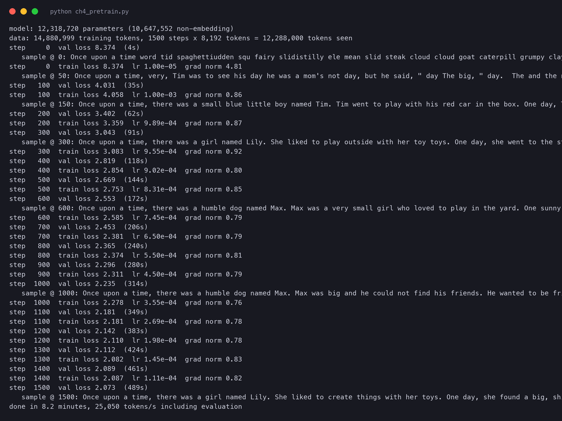
The curve has the shape of every pretraining curve:

1. A cliff in the first 100 steps (8.37 to 4.03). The model learns the cheapest lessons first: which tokens are common ("the", ".", " a") and which are never used. Just knowing the frequency of each token takes the loss from 8.3 to roughly the entropy of single tokens.
2. A long, bending slope (4.0 to 2.5 by step 600). The model learns word order, short phrases, then grammar.
3. A slow tail (2.5 to 2.07). Each further gain costs more steps, as the power laws of Section 4.7 predict. The decaying learning rate helps squeeze out the last part.

The training and validation curves lie on top of each other. That is expected when every token is seen once: the model has never seen the validation stories, but it has never seen most training stories more than once either, so there is nothing to overfit. In perplexity terms (Chapter 1), the final validation loss of 2.073 is $e^{2.073} = 7.95$: at each position the model is, on average, as unsure as if it were choosing uniformly among about 8 tokens, down from 4,096.

The samples tell the same story in words:

At step 600, "there was a humble dog named Max. Max was a very small girl" shows a model that has learned grammar and story templates but not yet to keep track of a character. At step 1,500, "there was a girl named Lily. She liked to create things with her toys. One day, she found a big, shiny thing in her room" keeps the same character and the right pronoun across sentences. Nobody told the model what a pronoun is: it is just the cheapest way to predict the next token in millions of stories.

4.12 What a base model learns#

Our tiny model learned a tiny world. A real base model, trained on trillions of tokens of web, books and code, learns a great deal more. ch4_probe.py probes Qwen2.5-0.5B, the base model of Chapter 1, without any fine-tuning, in three ways.

Facts#

The simplest probe gives the model the start of a factual sentence and looks at its five most likely next tokens:

'The capital of France is'                    ' Paris' 0.32  ' ______' 0.11  ' ____' 0.06  ' __' 0.06  ':\n' 0.05
'The chemical symbol for gold is'             ' ____' 0.37  ' __' 0.20  ' ______' 0.07  ' Au' 0.07  '\n' 0.04
'Romeo and Juliet was written by'             ' William' 0.33  ' Shakespeare' 0.17  ' the' 0.06  ' which' 0.05  ' a' 0.04
'The largest planet in the solar system is'   ' Jupiter' 0.45  ' the' 0.05  ' ' 0.04  ' Mercury' 0.03  ' __' 0.03

The facts are there: Paris, William (Shakespeare), Jupiter, Au. But look at the competitors. For "The chemical symbol for gold is", the most likely continuation is a blank, ____, with probability 0.37, and the right answer gets only 0.07. The model is not "trying to answer"; it is predicting what comes next in the kind of document that contains this sentence, and on the web a sentence like that most often appears in a fill-in-the-blank worksheet. A base model's knowledge and its behaviour are separate things. Fine-tuning (Chapter 5) changes the behaviour; it adds very little knowledge.

Grammar#

The second probe compares the log-probability of a right and a wrong continuation:

'The keys to the cabinet'            ' are'    -1.99   ' is'     -5.41   prefers the right one: True  (ratio 30.4x)
'The author of the books'            ' is'     -7.75   ' are'    -9.16   prefers the right one: True  (ratio 4.1x)
'Yesterday she'                      ' went'   -2.59   ' goes'   -9.33   prefers the right one: True  (ratio 841.8x)
'The children who live next door'    ' are'    -2.55   ' is'     -8.75   prefers the right one: True  (ratio 495.3x)
'I have never'                       ' seen'   -2.22   ' saw'    -8.01   prefers the right one: True  (ratio 324.8x)
'Each of the students'               ' has'    -5.22   ' have'   -9.69   prefers the right one: True  (ratio 86.6x)

All six are right, including the classic traps: "The keys to the cabinet" has a singular noun ("cabinet") right before the verb, but the subject is "keys", and the model prefers "are" 30 to 1. "Yesterday she" prefers the past tense "went" over "goes" by more than 800 to 1. The ratio is $e^{\log p_{\text{right}} - \log p_{\text{wrong}}}$; for the first line, $e^{-1.99 + 5.41} = e^{3.42} \approx 30$.

Our tiny TinyStories model learned the same kind of thing inside its small world:

'Lily and her mom went to the'                   ' park' 0.37  ' store' 0.16  ' kitchen' 0.07  ' beach' 0.02  ' shop' 0.02
'Tom was very sad because he lost his'           ' toy' 0.35  ' ball' 0.10  ' favorite' 0.05  ' friend' 0.04  ' red' 0.02
'The little girl smiled because she was very'    ' happy' 0.26  ' brave' 0.06  ' kind' 0.04  ' excited' 0.03  ' proud' 0.03

Every top-5 token is a noun after "the" or "his", and an adjective after "very"; and the meanings fit (sad because he lost his toy, smiled because she was happy).

In-context learning#

The most surprising thing pretraining produces was described in the GPT-3 paper: a large base model can learn a new task from examples in its prompt, with no change to its weights.

ch4_probe.py runs a small version of this experiment on Qwen2.5-0.5B with three tasks, 28 test items each, and 0, 1, 2, 4 or 8 examples in the prompt:

TASKS = {'English to French': (fr, ' ->', 'Translate English to French:\n'),
         'antonyms': (ant, ' ->', 'Write the opposite of each word:\n'),
         'sentiment with made-up labels (blue/red)': (senti, ' :', 'Label each review:\n')}
for name, (data, sep, head) in TASKS.items():
    pool, test = data[:8], data[8:]
    for k in [0, 1, 2, 4, 8]:
        shots = head + ''.join(f'{x}{sep} {y}\n' for x, y in pool[:k])
        correct = sum(answer(shots + f'{x}{sep}').lower().startswith(y) for x, y in test)

Each task has a one-line description, a separator, and a list of (input, answer) pairs. The first 8 pairs are the pool of examples, the rest are test items. For each k, the prompt is the description, k solved examples on separate lines, and then the new input followed by the separator; answer generates up to 6 tokens greedily and keeps the first line. The third task is the interesting one: reviews are labelled blue (positive) or red (negative). Those labels mean nothing; the model can only get them right by reading the examples.

English to French                          k=0: 43%  k=1: 86%  k=2: 82%  k=4: 86%  k=8: 82%   (28 test items)
antonyms                                   k=0: 36%  k=1: 93%  k=2: 89%  k=4: 82%  k=8: 89%   (28 test items)
sentiment with made-up labels (blue/red)   k=0: 0%  k=1: 54%  k=2: 4%  k=4: 100%  k=8: 100%   (28 test items)

For translation and antonyms, one example does most of the work: it shows the format, and the knowledge was already there. The made-up labels show genuine learning from the prompt: 0% with no examples (the model has never seen "blue" mean "positive"), and 100% with four. The steps in between are revealing. With one example (a positive review labelled "blue") the model answers "blue" for everything, which is right for the 15 positive reviews out of 28: 54%. With two examples, one "blue" and one "red", it got only 1 of 28 right. Asking it what it answers shows why:

what the model answers with only two labelled examples:
   'The view was beautiful' -> 'green'
   'The room was dirty' -> 'yellow'
   'Superb quality' -> 'green'

With two colours in the prompt, the 0.5B model decides it is reading a list of colours and continues the list. With four examples the pattern "positive review means blue" becomes the most likely reading. Small base models learn in context, but fragilely, which is one more reason to fine-tune them.

4.13 Data mixtures, mid-training and annealing#

The last ingredient is the one most model reports now spend the most pages on: which data, in what proportion, at which point of training.

Llama 3 describes its final pretraining mixture in one line, and then a technique that has become standard:

How do teams pick those proportions? The same way as everything else in this chapter: by training small models on candidate mixtures, measuring them, and using scaling laws to predict which mixture will be best at full scale. Llama 3 describes exactly that process for its data mix.

The Llama 3 paper also uses annealing as a cheap test: to judge whether a new small dataset is valuable, anneal a partly trained 8B model with 30% of the new data and 70% of the usual mix, and compare benchmark scores. That is far cheaper than a full training run per candidate dataset.

Between the main phase and the annealing, many recent models add a stage often called mid-training.

For Llama 3 405B, the long-context stage is an example: after the main phase, the context window was raised from 8K to 128K tokens in six steps, using about 800B tokens of training. Putting it together:

4.14 Where this leaves us#

At the end of pretraining you have a base model: a network that has compressed trillions of tokens into a few billion numbers, that knows facts and grammar, and that can pick up a task from a few examples. You have also seen its limits. It completes "The chemical symbol for gold is" with a blank because worksheets do. Asked a question, it might answer, continue with three more questions, or start a quiz. It has no notion of a user, of a turn, or of when to stop.

Turning this into a model that follows instructions does not need anything like the compute of pretraining. It needs a much smaller amount of the right data, and a few careful changes to the same loss. That is the subject of Chapter 5.

References#

Papers#

• Penedo, G. et al. (2024). The FineWeb Datasets: Decanting the Web for the Finest Text Data at Scale. arXiv:2406.17557
• Gao, L. et al. (2020). The Pile: An 800GB Dataset of Diverse Text for Language Modeling. arXiv:2101.00027
• Rae, J. W. et al. (2021). Scaling Language Models: Methods, Analysis & Insights from Training Gopher. arXiv:2112.11446
• Raffel, C. et al. (2019). Exploring the Limits of Transfer Learning with a Unified Text-to-Text Transformer (C4). arXiv:1910.10683
• Penedo, G. et al. (2023). The RefinedWeb Dataset for Falcon LLM. arXiv:2306.01116
• Li, J. et al. (2024). DataComp-LM: In search of the next generation of training sets for language models. arXiv:2406.11794
• Lee, K. et al. (2022). Deduplicating Training Data Makes Language Models Better. arXiv:2107.06499
• Sennrich, R., Haddow, B. and Birch, A. (2016). Neural Machine Translation of Rare Words with Subword Units. arXiv:1508.07909
• Vaswani, A. et al. (2017). Attention Is All You Need. arXiv:1706.03762
• Kaplan, J. et al. (2020). Scaling Laws for Neural Language Models. arXiv:2001.08361
• Hoffmann, J. et al. (2022). Training Compute-Optimal Large Language Models (Chinchilla). arXiv:2203.15556
• Besiroglu, T. et al. (2024). Chinchilla Scaling: A replication attempt. arXiv:2404.10102
• Brown, T. et al. (2020). Language Models are Few-Shot Learners (GPT-3). arXiv:2005.14165
• Grattafiori, A. et al. (2024). The Llama 3 Herd of Models. arXiv:2407.21783
• Qwen Team (2024). Qwen2.5 Technical Report. arXiv:2412.15115
• Hu, S. et al. (2024). MiniCPM: Unveiling the Potential of Small Language Models with Scalable Training Strategies (warmup-stable-decay). arXiv:2404.06395
• Loshchilov, I. and Hutter, F. (2019). Decoupled Weight Decay Regularization (AdamW). arXiv:1711.05101
• Micikevicius, P. et al. (2018). Mixed Precision Training. arXiv:1710.03740
• Eldan, R. and Li, Y. (2023). TinyStories: How Small Can Language Models Be and Still Speak Coherent English? arXiv:2305.07759

Other sources#

• Common Crawl, the open web archive used in Section 4.2. commoncrawl.org
• The FineWeb-Edu classifier used in ch4_data.py. huggingface.co/HuggingFaceFW/fineweb-edu-classifier
• The TinyStories dataset used in Section 4.11. huggingface.co/datasets/roneneldan/TinyStories
• The scripts behind every number in this chapter: code/training/ch4_*.py, with their saved output in code/training/results/.