Beyond One GPU: Tensor, Pipeline and Expert Parallelism, and Split Prefill and Decode
Why big models need many GPUs, what the wires between them cost, and how tensor, pipeline and expert parallelism and disaggregated serving split the work: a real two-process tensor-parallel run, measured MoE routing, and worked arithmetic.
Llama 3.1 70B stores its weights in 141 GB. A widely used data-centre GPU, the NVIDIA H100, has 80 GB of memory. The model does not fit, and nothing clever inside one GPU changes that.
So we split the model across several GPUs. The moment we do, a new cost appears that the first six parts of this series could ignore: the GPUs have to talk to each other, many times for every single token. How often they talk, how much they send, and how fast the wire between them is, decides almost everything about how a model should be spread out.
This part builds the whole picture from the ground up:
- Why one GPU is not enough: the memory arithmetic for an 8B, a 70B, a 405B and a 671B model, and the speed limit on decode.
- The wires: how fast GPUs can talk inside one server and between servers, and a simple model of what a message costs.
- Tensor parallelism: split every layer across GPUs. We run a real model this way, in two separate processes that only share numbers through a sum, and check it gives the same answer.
- Collectives: all-reduce, all-gather and all-to-all, the few ways a group of GPUs exchange data, with the cost formula worked out.
- Pipeline parallelism: give each GPU a slice of the layers instead.
- Expert parallelism for mixture-of-experts models, with real routing decisions recorded from a 64-expert model.
- Disaggregated prefill and decode: run the two phases from Part 1 on different GPUs, and move the KV cache between them.
- The real systems that do this today, and the flags you would set.
- How to choose a layout, with worked examples.
This part builds on Part 6 (coming soon), which covered serving on one GPU per copy of the model: latency targets, goodput, queueing, capacity planning and routing between copies. Here we look inside a copy that is too big for one GPU.
1. Why one GPU is not enough
Memory: weights plus the KV cache
A GPU must hold two big things while it serves a model:
- the weights, read on every forward pass (Part 1);
- the KV cache, the saved keys and values of every token of every conversation in flight (Part 2).
The weight size is the number of parameters times the bytes per parameter. The KV cache size is the formula from Part 2:
where:
- is the number of parameters and the bytes per parameter (2 for BF16, 1 for FP8);
- is the number of layers, the number of key-value heads and the size of each head;
- the 2 counts keys and values, and is the bytes per stored number (2 for BF16);
- is the number of conversations being served at once and the tokens in each one.
Worked example: Llama 3.1 70B. The Llama 3 report gives 80 layers, 8 KV heads and a model width of 8,192 (64 heads of 128). Counting every matrix gives billion, so the weights take GB. One token of KV cache is bytes, 320 KiB. Serve 32 conversations of 8,192 tokens and the cache is GiB. Together that is 227 GB. With about 90% of each 80 GB GPU usable (the rest goes to the CUDA runtime, activations and fragmentation), that needs four H100s.
The same arithmetic for the other models:
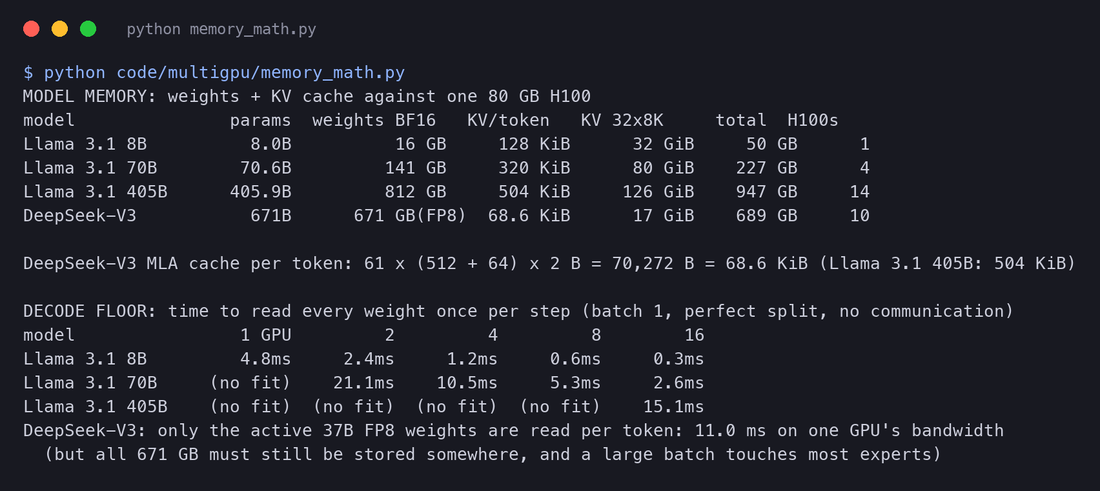
Three things stand out.
The 8B model fits on one GPU with room to spare. For it, more GPUs mean more copies of the model, not a split model. That is the world of Part 6.
The 405B model does not even fit on one 8-GPU server. In BF16 its weights alone are 812 GB, more than the 640 GB of eight H100s. Meta hit exactly this wall:
DeepSeek-V3 is bigger but its cache is smaller. It has 671 billion parameters, stored in FP8 (one byte each), so 671 GB. But it uses multi-head latent attention (MLA, mentioned in Part 2): each layer caches one compressed vector of 512 numbers plus a 64-number position key, shared by all heads. That is bytes per token, 68.6 KiB, against 504 KiB for Llama 3.1 405B. Its problem is the weights, not the cache.
Speed: decode is limited by reading the weights
Even when a model fits, there is a second reason to spread it: speed. Part 1 showed that a decode step for a small batch is memory-bound: the GPU spends its time reading every weight once, not multiplying. That gives a hard floor on the time per token:
where:
- is the size of the weights in bytes;
- is the number of GPUs the weights are split over, each reading only its own share;
- is one GPU's memory bandwidth (3.35 TB/s for an H100).
Worked example. Llama 3.1 70B on 2 H100s: ms, at best 47 tokens per second for one user. On 8 H100s each GPU reads only 17.6 GB, so the floor drops to 5.3 ms. Spreading the weights does not just make the model fit; it multiplies the memory bandwidth working on each token.
That last condition, "if communication were free", is the whole subject of this article. It is not free.
2. The wires between GPUs
Inside a server and between servers
A typical AI server (NVIDIA calls it a node) has eight GPUs. They are connected to each other in two very different ways, depending on whether the other GPU is in the same box.
Put the numbers side by side:
| Link | Peak bandwidth | Compared with NVLink |
|---|---|---|
| HBM, inside one H100 | 3,350 GB/s | (the GPU's own memory) |
| NVLink 4, GPU to GPU in a server | 900 GB/s both ways (450 each way) | 1x |
| PCIe Gen5 x16 | 128 GB/s both ways (64 each way) | 7x slower |
| InfiniBand NDR, one 400 Gb/s card | 50 GB/s each way | 9x slower |
| Ethernet, 100 Gb/s | 12.5 GB/s each way | 36x slower |
These are NVIDIA's published peaks (the H100 page lists "NVIDIA NVLink: 900GB/s" and "PCIe Gen5: 128GB/s"; the ConnectX-7 page lists 400 Gb/s). The newer Blackwell generation doubles NVLink to 1,800 GB/s per GPU and can join 72 GPUs into one NVLink domain (the "NVL72" racks), which moves the line between "inside" and "outside" further out. The shape of the problem stays the same.
Real clusters see less than peak. DeepSeek reports what their H800 cluster (a version of the H100 with reduced NVLink bandwidth, made for export to China) delivers in practice:
What one message costs: latency plus size over bandwidth
Every message between GPUs costs a fixed amount of time before any data moves (setting up, synchronising, crossing switches), plus time proportional to its size. This is called the alpha-beta model:
where:
- is the message size in bytes;
- (alpha) is the fixed cost per message, in seconds;
- (beta) is the bandwidth in bytes per second.
Worked example. Send 16 KiB (16,384 bytes) over NVLink at 450 GB/s each way. The size term is ns. If the fixed cost is a few microseconds (an assumed figure; NVIDIA does not publish one), it is about 100 times bigger than the data term. Small messages are all alpha; large messages are all beta.
NVIDIA does not publish an alpha for NVLink or InfiniBand, and I cannot measure one without the hardware. So I measured the shape on what I have: separate processes on this laptop's CPU, exchanging data with torch.distributed (the same library NVIDIA GPUs use, but with its CPU backend, called gloo).
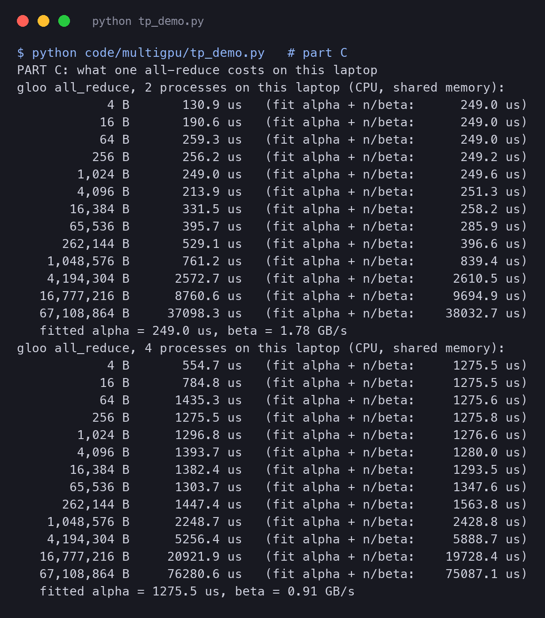
The curve is flat for small messages and then rises in step with size: exactly . On this laptop the flat part is about 0.25 ms with 2 processes and 1.3 ms with 4: more participants means more steps and more waiting for the slowest one, a first hint of Section 4. (These alphas are hundreds of times larger than a GPU's, because they are CPU processes on a busy machine; only the shape carries over.) The flat part is why the next sections keep asking two separate questions about every design: how many messages per token, and how many bytes per message.
3. Tensor parallelism: split every layer
The idea
Tensor parallelism attacks both problems from Section 1 at once: each GPU stores of the weights, and each GPU reads only of them per step. The price is communication inside every layer. The trick, from the Megatron-LM paper (Shoeybi et al., 2019), is to cut the matrices so that the communication happens as rarely as possible.
Splitting the MLP: columns, then rows
A transformer's MLP block is two matrix multiplications with a nonlinearity between them:
where:
- is the input, one row per token, columns wide (the model width);
- is a weight matrix that widens each token to numbers (the FFN width);
- GeLU is the nonlinear function applied to every number (Llama uses a close cousin, SwiGLU);
- is an matrix that narrows each token back to numbers.
There are two ways to cut in half. Megatron's authors explain why only one of them works well:
Written out for two GPUs, with split by columns and split by rows:
The GeLU is applied to each column of separately, so it does not care how the columns are grouped. The only cross-GPU step is the final +.
Check it: the sum of the parts equals the whole
This is easy to verify. The first part of tp_demo.py builds an MLP with Qwen2.5-0.5B's sizes (, ), splits it two, four and eight ways, and compares the sum of the pieces with the unsplit result:
full = F.gelu(X @ A) @ B
for p in [2, 4, 8]:
    A_parts = A.chunk(p, dim=1)              # column split: each GPU gets ffn/p output columns
    B_parts = B.chunk(p, dim=0)              # row split: each GPU gets the matching ffn/p rows
    partial = [F.gelu(X @ Ai) @ Bi for Ai, Bi in zip(A_parts, B_parts)]   # no communication needed here
    Y = sum(partial)                         # the all-reduce: add the p partial outputs
    res[p] = float((Y - full).abs().max())
chunk(p, dim=1) cuts into blocks of columns; chunk(p, dim=0) cuts into the matching blocks of rows. Each list entry in partial is what one GPU would compute on its own. sum(partial) is the all-reduce. Then the wrong way, splitting by rows and applying GeLU before adding:
Xs, As = X.chunk(2, dim=1), A.chunk(2, dim=0)
wrong = sum(F.gelu(Xi @ Ai) for Xi, Ai in zip(Xs, As)) @ BPART A: split matrix multiplies (float64, CPU)
p=2: each part A_i (896, 2432), B_i (2432, 896); max |sum of parts - unsplit| = 1.1e-14
p=4: each part A_i (896, 1216), B_i (1216, 896); max |sum of parts - unsplit| = 1.3e-14
p=8: each part A_i (896, 608), B_i (608, 896); max |sum of parts - unsplit| = 1.2e-14
row-split first matrix, GeLU applied before adding: max error 0.909 (output values are about 0.533 on average) -> needs a sync before GeLUThe column-then-row split matches the unsplit result to , which is just the rounding of 64-bit floats. The row split is wrong by more than the size of the answer itself, because . To use it you would have to add the halves before the GeLU: a second all-reduce per layer.
Splitting attention: whole heads per GPU
Attention splits even more naturally. Its heads are already independent: head 3 never looks at head 5's numbers until the output projection mixes them. So each GPU takes a whole group of heads, with their query, key and value weights (a column split), and the matching rows of the output projection (a row split). Again one all-reduce adds the partial outputs.
There is a bonus: each GPU only caches the keys and values of its own heads. The KV cache is split ways along with the weights, so the room for conversations grows with every GPU you add.
There is also a limit. With grouped-query attention (Part 2), Llama 3.1 70B has 64 query heads but only 8 KV heads. At TP=8 each GPU gets exactly one KV head. At TP=16 two GPUs would need the same KV head, so it must be copied, and the cache stops shrinking. That is one reason tensor parallelism usually stops at the 8 GPUs of one server.
The paper's own picture shows both blocks. The boxes marked and are where communication happens; in the forward pass does nothing and is the all-reduce:
A real tensor-parallel run, in two processes
Splitting one MLP is a toy. To be sure the whole recipe works, tp_demo.py runs all 24 layers of Qwen2.5-0.5B with tensor parallelism across two separate operating-system processes. Each process loads the model, keeps only its own half of every layer, and the two talk only through torch.distributed.all_reduce, the same call vLLM and SGLang make on NVIDIA GPUs (here with the CPU backend, gloo, since there is no NVIDIA GPU). Qwen2.5-0.5B has 14 query heads and 2 KV heads, so with TP=2 each process gets 7 query heads and 1 KV head.
Each process slices its share of the weights once, at load time:
qs = slice(rank * self.hq * hd, (rank + 1) * self.hq * hd)     # this rank's query heads
ks = slice(rank * self.hkv * hd, (rank + 1) * self.hkv * hd)   # this rank's KV heads
fs = slice(rank * ffn, (rank + 1) * ffn)                       # this rank's MLP hidden units
self.layers.append(dict(
    wq=g('self_attn.q_proj.weight')[qs], bq=g('self_attn.q_proj.bias')[qs],      # column split
    wk=g('self_attn.k_proj.weight')[ks], bk=g('self_attn.k_proj.bias')[ks],
    wv=g('self_attn.v_proj.weight')[ks], bv=g('self_attn.v_proj.bias')[ks],
    wo=g('self_attn.o_proj.weight')[:, qs],                                        # row split
    wg=g('mlp.gate_proj.weight')[fs], wu=g('mlp.up_proj.weight')[fs],              # column split
    wd=g('mlp.down_proj.weight')[:, fs]))                                          # row split
PyTorch stores a linear layer's weight as (output, input), so a column split of the maths is a slice of the weight's first axis ([qs]), and a row split is a slice of its second axis ([:, qs]). The gate and up projections of Qwen's SwiGLU MLP are both column-split the same way, so their elementwise product stays local.
Then each layer of the forward pass is ordinary code, with exactly two collective calls:
a = F.scaled_dot_product_attention(q, K, V, is_causal=ids.shape[0] > 1)   # my 7 heads only
a = a.transpose(0, 1).reshape(ids.shape[0], -1)
h = h + self.all_reduce(a @ L['wo'].T)       # all-reduce 1 of 2 in this layer
x = rms(h, L['ln2'], c.rms_norm_eps)
m = F.silu(x @ L['wg'].T) * (x @ L['wu'].T)  # my half of the MLP
h = h + self.all_reduce(m @ L['wd'].T)       # all-reduce 2 of 2 in this layer
self.all_reduce wraps dist.all_reduce, which replaces each process's tensor with the sum over both processes, and counts the calls and bytes. Everything outside the two calls (embeddings, normalisation, the residual additions, the output head) is simply done on both processes, which is how Megatron handles them too (it can also split the vocabulary, which this demo skips).
The script compares the last-token logits with the unsplit Hugging Face model and greedily generates 24 tokens both ways:
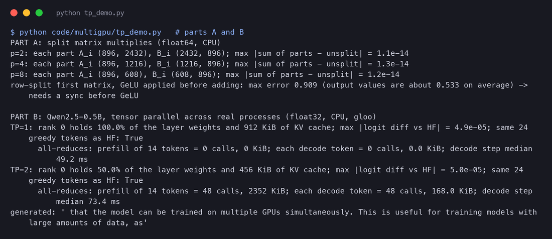
The split model gives the same 24 tokens as the original, and the logits agree to about , the same small difference that the unsplit re-implementation has (float32 sums in a different order). Each process holds exactly half of the layer weights and half of the KV cache. And every decode token costs 48 all-reduces: 24 layers times two.
The timings in that run are not a speed-up: both "GPUs" are processes on one CPU, sharing the same cores and memory, so splitting gives each process half the work but no extra hardware to do it with. This demo checks correctness and counts messages; the next pages estimate speed.
How many bytes per token?
Each all-reduce carries one activation vector per token: numbers. Per decode step:
where:
- is the number of layers (two all-reduces each);
- is the number of tokens in the step (the batch size during decode);
- is the model width and the bytes per number (2 for BF16).
Worked example, Qwen2.5-0.5B in the demo: calls, each bytes in float32, so bytes = 168 KiB per token, exactly the 168.0 KiB the script counted.
Worked example, Llama 3.1 70B in BF16: all-reduces per step. At batch 1 each carries KiB; at batch 64, 1 MiB. Compare that with what each GPU reads from its own memory at TP=8: 17.6 GB of weights. The bytes sent are tiny next to the bytes read. But there are 160 separate messages, and each must finish before the layer can go on. From Section 2: when messages are small, it is their count, through , that costs time.
What each GPU's share costs: a measurement
To see how the work per GPU shrinks, measure_mps.py times one real Llama 3.1 8B MLP matrix (14,336 by 4,096, BF16, 117 MB) on this laptop's Apple GPU, whole and cut to the half and quarter that TP=2 and TP=4 would give each GPU:
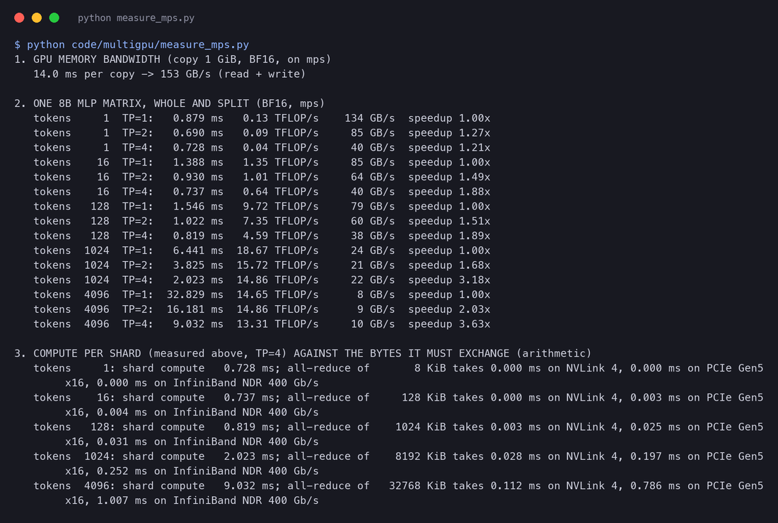
Two regimes show up. With 4,096 tokens the work is arithmetic, and the shards behave as hoped: the half takes half the time (2.03x faster) and the quarter close to a quarter (3.63x). With one token, the whole matrix is a 117 MB read at 134 GB/s, 0.88 ms. But the half and quarter shards take 0.69 and 0.73 ms, barely faster. Below a certain size, every GPU operation has a fixed cost of its own (launching the kernel and getting it going), and splitting the work cannot go under that floor. It is the same shape as the alpha of Section 2, inside one GPU. Engines fight it by capturing a whole decode step as one CUDA graph, so that hundreds of small launches cost about one; the principle stays: cutting small work very finely gives diminishing returns, even before any communication.
The last block of the output adds the communication those shards would need: the partial outputs are only 8 KiB per token, which takes nanoseconds on any link. The bytes are not the problem; the number of separate exchanges is. (The copy bandwidth here, 153 GB/s, is lower than the 262 GB/s measured in Part 1 because this run shared the laptop with other jobs; the fastest of 40 runs is reported for every number.)
Putting it together: TP on 70B
Now add the communication back. layout_model.py estimates one Llama 3.1 70B decode step on H100s as the time to read the weights and the KV cache (or to do the arithmetic, whichever is longer) plus 160 all-reduces:
where:
- is the weight bytes and the KV-cache bytes read in the step ( sequences of 4,096 tokens each);
- is one GPU's peak BF16 rate (989 TFLOP/s for an H100) and the arithmetic for tokens;
- the last term is all-reduces, each costing two message delays () plus its bytes, using the two-step all-reduce explained in Section 4, with = 450 GB/s;
- s is an assumption (NVIDIA publishes none); it is varied below.
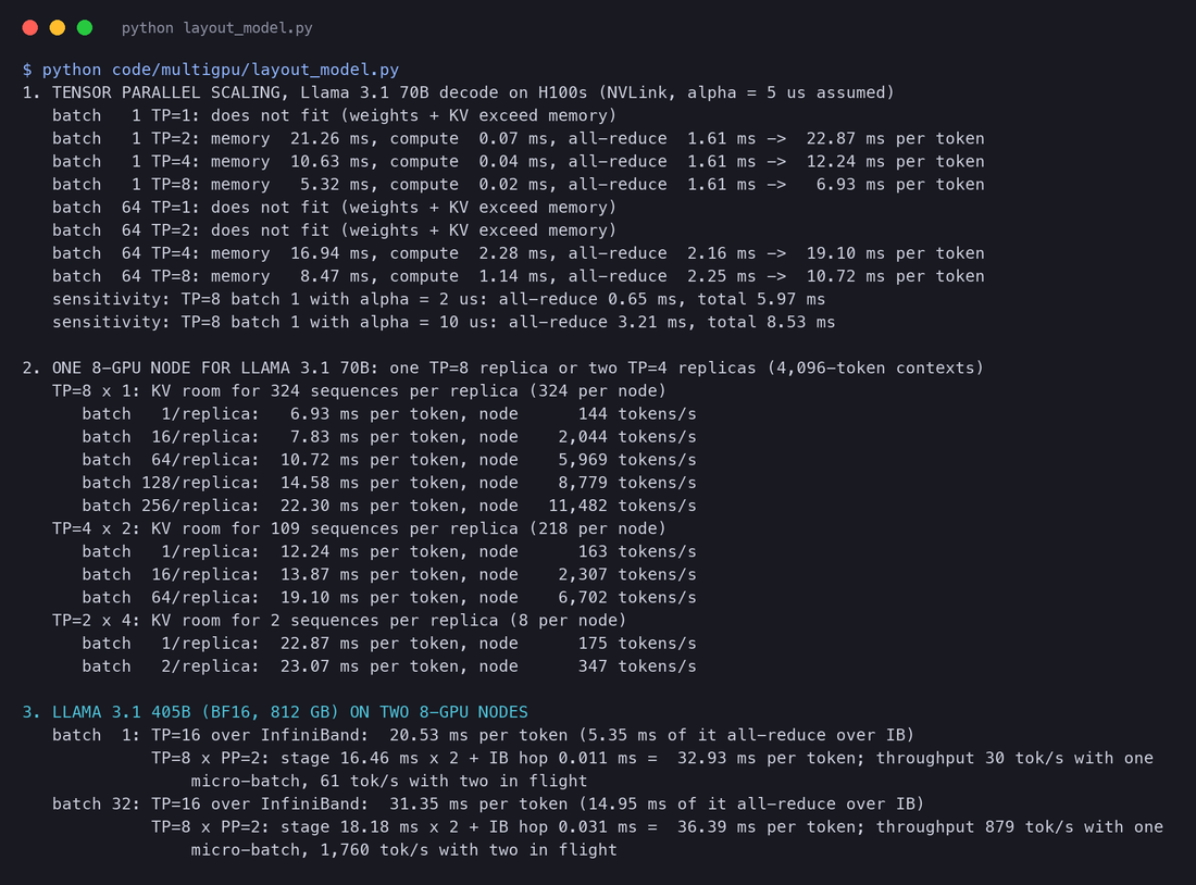
Worked example at batch 1. TP=2: reading 141 GB at TB/s takes 21.3 ms (with the cache); 160 all-reduces at each add 1.6 ms; total 22.9 ms. TP=8: memory 5.3 ms, all-reduces still 1.6 ms, total 6.9 ms. Going from 2 to 8 GPUs cut the memory time by 4x but left the communication exactly where it was, so the step is only 3.3x faster, and communication grew from 7% to 23% of it. With s the TP=8 step is 6.0 ms; with s it is 8.5 ms.
This is a general law, and the Google team that scaled PaLM inference put it plainly:
Two practical consequences follow. Tensor parallelism belongs where is small and links are fast: inside one NVLink server. And because it needs that, inference engines put real effort into making all-reduce fast: vLLM and TensorRT-LLM ship their own all-reduce kernels for small messages on NVLink, rather than relying only on the general NCCL library. Section 4 shows why that helps.
4. Collectives: how a group of GPUs exchanges data
The four you need
When a group of GPUs exchange data in a fixed pattern, the operation is called a collective. NVIDIA's NCCL library (pronounced "nickel") implements them on GPUs; torch.distributed calls it. Four collectives cover almost everything in this article.
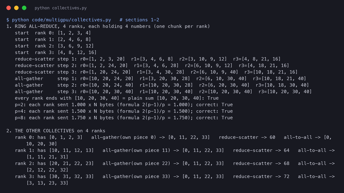
collectives.py runs all four on four simulated GPUs (list entries in NumPy), where rank starts with :
Ring all-reduce, step by step
How do GPUs compute a sum without one GPU becoming a bottleneck? The classic answer is the ring. Arrange the GPUs in a circle and cut each vector into chunks.
- Reduce-scatter, steps. At each step every GPU sends one chunk to its right-hand neighbour, which adds it to its own copy of that chunk. After steps, each GPU holds one chunk that contains the complete sum.
- All-gather, more steps. Each GPU passes its finished chunk to the right, and the finished chunks travel round the ring until everyone has all of them.
Here is the trace for four ranks holding times 1, 2, 3 and 4:
What the ring costs
Each step moves one chunk, bytes, from every GPU at the same time. There are steps. So, with the alpha-beta model from Section 2:
where:
- is the number of GPUs and the size of the vector being summed, in bytes;
- is the fixed cost of one step and each GPU's sending bandwidth.
The byte term is the famous property of the ring: each GPU sends times the vector, which is never more than 2x the vector however many GPUs there are. The simulation counts the bytes and agrees: 1.000, 1.500 and 1.750 times for 2, 4 and 8 ranks. (NCCL's performance notes use the same factor to turn measured times into "bus bandwidth".)
The latency term is the catch. It grows with : steps on 8 GPUs, and every GPU must wait for its neighbour at every step.
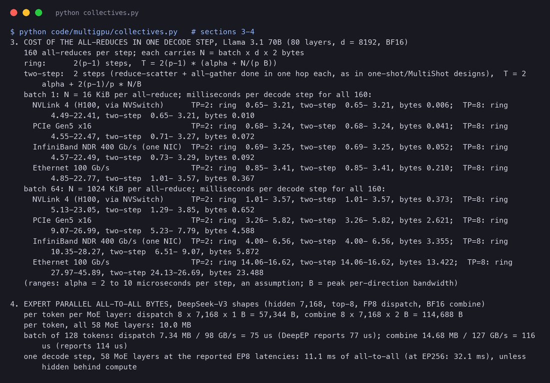
Worked example: Llama 3.1 70B at batch 1, TP=8, NVLink. Each all-reduce carries KiB. Bytes: ns. Latency: , so to s for between 2 and 10 s. Times 160 all-reduces: 4.5 to 22.4 ms per token, while the bytes alone would take 0.01 ms. A ring is the wrong shape for tiny messages.
Fewer steps for small messages
That is why there are other algorithms. With NVSwitch every GPU can reach every other directly, so a GPU can send each peer its chunk in one step (a one-hop reduce-scatter) and then gather the sums in one more step: two steps, whatever is. NVIDIA describes this for TensorRT-LLM (their "MultiShot" all-reduce, which uses the switch to multicast):
"This process is repeated 2N-2 times where N is the number of GPUs working together ... This increases latency, as all GPUs need to stay synchronized at every step of the ring." (NVIDIA technical blog, 3x Faster AllReduce with NVSwitch and TensorRT-LLM MultiShot, November 2024)
The two-step version costs about
with the same symbols as before. Same bytes, but only two delays. For the 70B example: = 0.65 to 3.2 ms per token, about 7x less than the ring at TP=8. (NCCL itself also switches algorithm and protocol by message size; the point is that small all-reduces are a latency problem, and good implementations attack the step count.)
| Llama 3.1 70B, all 160 all-reduces of one decode step | Ring | Two-step | Bytes only |
|---|---|---|---|
| TP=2, batch 1, NVLink | 0.65 to 3.21 ms | 0.65 to 3.21 ms | 0.006 ms |
| TP=8, batch 1, NVLink | 4.49 to 22.41 ms | 0.65 to 3.21 ms | 0.010 ms |
| TP=8, batch 64, NVLink | 5.13 to 23.05 ms | 1.29 to 3.85 ms | 0.65 ms |
| TP=8, batch 64, PCIe Gen5 | 9.07 to 26.99 ms | 5.23 to 7.79 ms | 4.59 ms |
| TP=8, batch 64, one 400 Gb/s NIC | 10.35 to 28.27 ms | 6.51 to 9.07 ms | 5.87 ms |
Ranges are for = 2 to 10 s (assumed); bandwidths are per-direction peaks. Read the table by rows:
- At batch 1 the bytes never matter; only the number of steps does.
- At batch 64 the bytes start to count, and on PCIe or the network they alone cost 4.6 to 5.9 ms per token, as much as reading the weights. That is why the vLLM documentation tells you to avoid tensor parallelism on GPUs without NVLink (Section 8).
5. Pipeline parallelism: split the layers instead
The idea, from training
Pipeline parallelism communicates far less than tensor parallelism. Between two stages it sends the activations once ( bytes, point to point), instead of two all-reduces in every layer. The cost is idle time. GPipe (Huang et al., 2019) introduced the standard picture:
GPipe gives the size of the bubble:
Worked example. stages. With : idle. With : .
Pipelines during decode
Decode adds a twist: the next token of a sequence cannot start until its previous token has left the last stage. One sequence alone keeps only one stage busy at a time. Several independent groups of sequences (micro-batches) fill the gaps. layout_model.py lays out the schedule for 4 stages, each micro-batch generating 3 tokens:
The figure shows the two faces of pipelining:
- Throughput improves with micro-batches: 12 tokens in 15 slots instead of 3 tokens in 12.
- Latency does not. Each token still passes through all 4 stages one after another, each stage running only its quarter of the layers. A pipeline never makes one sequence's token faster than reading all its layers on one GPU would, and it adds a network hop between stages.
Meta's choice for Llama 3 405B, from the same section as the box in Section 1, follows from this:
Worked example: 405B on two nodes
layout_model.py compares two ways to use 16 H100s in two nodes for Llama 3.1 405B:
- TP=16: every layer split 16 ways, so 252 all-reduces per step, all crossing InfiniBand ( assumed 10 s, = 50 GB/s per GPU).
- TP=8 x PP=2: each node holds 63 layers, split 8 ways over NVLink; one hop over InfiniBand per step.
| Batch 32 | ms per token | Tokens per second |
|---|---|---|
| TP=16 across both nodes | 31.4 (15.0 of it all-reduce over InfiniBand) | 1,020 |
| TP=8 x PP=2, one micro-batch | 36.4 | 879 |
| TP=8 x PP=2, two micro-batches | 36.4 | 1,760 |
Per token, the pipeline is slower: each token reads 406 GB on 8 GPUs (15.1 ms) in the first node, then again in the second, plus the hop. TP=16 reads everything in parallel on 16 GPUs but spends almost half its time in all-reduces over the network. Fill the pipeline with two micro-batches and it delivers 1.7x the throughput of TP=16 while sending a few kilobytes per token over InfiniBand instead of hundreds of messages. If latency matters most and the network is excellent, TP across nodes can win; for throughput per GPU, the pipeline does. Both conclusions depend on the assumed , which is why the code keeps it as a named input.
6. Expert parallelism for mixture-of-experts models
Why MoE models need their own kind of parallelism
A mixture-of-experts layer replaces one big MLP with many small ones. DeepSeek-V3 has, in each of its 58 MoE layers, 256 routed experts (each an MLP with a hidden width of 2,048) plus one shared expert that every token uses. A small router scores the experts for each token and sends the token to its top 8.
You could split every expert with tensor parallelism. But each expert is small, and an all-reduce per expert per layer would be pure overhead. The natural move is the opposite: keep each expert whole and give different experts to different GPUs.
Each MoE layer then runs in four stages:
- Each GPU runs attention for its own tokens, and the router picks each token's experts.
- Dispatch: an all-to-all sends each token's activations to the GPUs that hold its experts.
- Each GPU runs its experts on whatever tokens it received.
- Combine: a second all-to-all sends the outputs back, where they are added with the router's weights.
How many bytes
Each token is sent once per chosen expert, and the answers come back the same way.
where:
- is the number of experts chosen per token (8 for DeepSeek-V3);
- is the model width (7,168);
- and are the bytes per number on the way out and back: DeepSeek sends 1 byte (FP8) out and 2 bytes (BF16) back.
Worked example. bytes per token per layer; over 58 MoE layers, 10.0 MB per token. A decode batch of 128 tokens per GPU dispatches MB per layer.
DeepSeek's open-source all-to-all library, DeepEP, published timings for exactly this setting (H800s with 400 Gb/s InfiniBand, 128 tokens per batch, hidden 7,168, top-8, FP8 dispatch, BF16 combine; README of release v1.2.1). Our byte count reproduces them: 7.34 MB at their measured 98 GB/s is 75 s, against the 77 s they report for EP8 dispatch; 14.68 MB of combine at 127 GB/s is 116 s against 114 s reported. Across all 58 MoE layers that is 11.1 ms per decode step at EP8 and 32.1 ms at EP256 (194 and 360 s per layer), unless it is hidden behind computation. That is why DeepSeek runs two micro-batches and overlaps one's communication with the other's compute.
The real problem: load imbalance
All-to-all has a second cost that the bytes do not show. A layer is finished only when the busiest GPU is finished. If the router sends twice the average number of tokens to the experts on one GPU, that GPU takes twice as long and every other GPU waits.
How uneven is real routing? Rather than guess, moe_routing.py records it. It runs the real OLMoE-1B-7B model (64 experts per layer, 8 chosen per token, 16 layers, 6.9 billion parameters) on this laptop's GPU over 12,288 tokens of WikiText and 12,288 tokens of Python code, and saves which 8 experts the router chose for every token in every layer. That is about 3 million real routing decisions. The routing is the measurement; nothing is timed.
The recording is a forward hook on each layer's router, which returns the chosen expert ids as its third output:
for i, layer in enumerate(model.model.layers):
    hooks.append(layer.mlp.gate.register_forward_hook(
        lambda m, inp, out, i=i: buf.setdefault(i, []).append(out[2].cpu())))
with torch.no_grad():
    for s in seqs:
        model(torch.tensor(s, device=dev)[None])
Then plain Python asks what those choices would do to expert parallelism. Experts to are placed in order, per GPU, and for random batches of tokens we compute the load on the busiest GPU divided by the average load:
counts = np.bincount(picks[l, idx].ravel(), minlength=E)   # tokens sent to each expert in this batch
load = np.zeros(n_gpus)
np.add.at(load, expert_to_gpu, counts)                       # tokens each GPU must process
ratios.append(load.max() / load.mean())                      # 1.00 = perfectly even
The same calculation on random routing (each token picks 8 experts uniformly) separates bad luck from real preference.
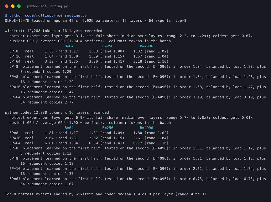
First, the experts themselves. In a typical layer the busiest expert receives 3.1 times its fair share of WikiText tokens (2.2x to 4.2x across layers), and on code 6.9 times; the idlest receive almost nothing.
Then what that does to GPUs:
| Busiest GPU / average, batches of 4,096 tokens | EP=8 | EP=16 | EP=64 |
|---|---|---|---|
| Random routing (chance only) | 1.02 | 1.04 | 1.10 |
| Real routing, WikiText | 1.32 | 1.57 | 3.18 |
| Real routing, Python code | 1.80 | 2.61 | 6.77 |
Three lessons:
- Big batches do not save you. Random imbalance fades as batches grow (1.17 at 64 tokens, 1.02 at 4,096 for EP=8). Real imbalance does not (1.35 and 1.32): it comes from the router's genuine preferences, not from small numbers.
- Wider EP makes it worse. At EP=64 each GPU holds one expert, so the busiest GPU is simply the hottest expert: 3.2x the average on WikiText, 6.8x on code. Two thirds or more of the GPU time in the layer is waiting.
- The hot experts depend on the traffic. WikiText and code share a median of 1 of their 8 hottest experts per layer. A placement tuned on yesterday's chat traffic can be wrong for today's coding traffic.
(OLMoE was trained with a load-balancing loss, like most MoE models, and DeepSeek-V3 adds its own auxiliary-loss-free balancing. Training reduces the skew, but as these numbers show, it does not remove it at serving time, when the mix of text is whatever users send.)
The fix: place experts by load, and copy the hot ones
DeepSeek's report describes what they do in production:
moe_routing.py tries the same two ideas on OLMoE's routing. It learns from the first half of the recorded tokens and is tested on the second half, just as a server must use past load to plan for future load:
- Placement by load: put the heaviest experts first, each on the least-loaded GPU that still has room.
- Redundant copies: each GPU gets a few spare slots; repeatedly copy the busiest expert on the busiest GPU to the least-loaded GPU with a free slot (keeping a copy only if it does not create a new busiest GPU), and split that expert's tokens evenly between its copies.
| Busiest / average, tested on unseen tokens | In order | Placed by load | Plus redundant copies |
|---|---|---|---|
| WikiText, EP=8 (8 copies) | 1.34 | 1.28 | 1.29 |
| WikiText, EP=16 (16 copies) | 1.58 | 1.47 | 1.47 |
| WikiText, EP=64 (64 copies) | 3.19 | 3.19 | 2.77 |
| Code, EP=8 (8 copies) | 1.81 | 1.12 | 1.12 |
| Code, EP=16 (16 copies) | 2.62 | 1.74 | 1.37 |
| Code, EP=64 (64 copies) | 6.75 | 6.75 | 1.67 |
When a GPU holds several experts, placing them by load does most of the work (code at EP=8: 1.81 to 1.12). When a GPU holds only one expert, placement cannot help at all, and only copies help (code at EP=64: 6.75 to 1.67). The leftover imbalance on WikiText comes from the traffic changing between the two halves of the text, which is exactly why DeepSeek refreshes its choice every 10 minutes and is "exploring a dynamic redundancy strategy" (same section) that re-plans for every batch.
DeepSeek-V3 in production
Putting the pieces together, here is how DeepSeek serves V3, with prefill and decode on separate groups of machines (Section 7 explains why):
DeepSeek later published what this looks like in daily operation. Their inference system overview (February 2025) describes a slightly different production layout than the paper, EP32 for prefill over 4 nodes and EP144 for decode over 18 nodes, each with 32 redundant experts, and reports the results over one day:
![DeepSeek inference system overview: Prefilling Phase [Routed Expert EP32, MLA/Shared Expert DP32]: Each deployment unit spans 4 nodes with 32 redundant routed experts, where each GPU handles 9 routed experts and 1 shared expert. Decoding Phase [Routed Expert EP144, MLA/Shared Expert DP144]: Each deployment unit spans 18 nodes with 32 redundant routed experts, where each GPU manages 2 routed experts and 1 shared expert.](/img/multigpu/deepseek-day6-units.png)
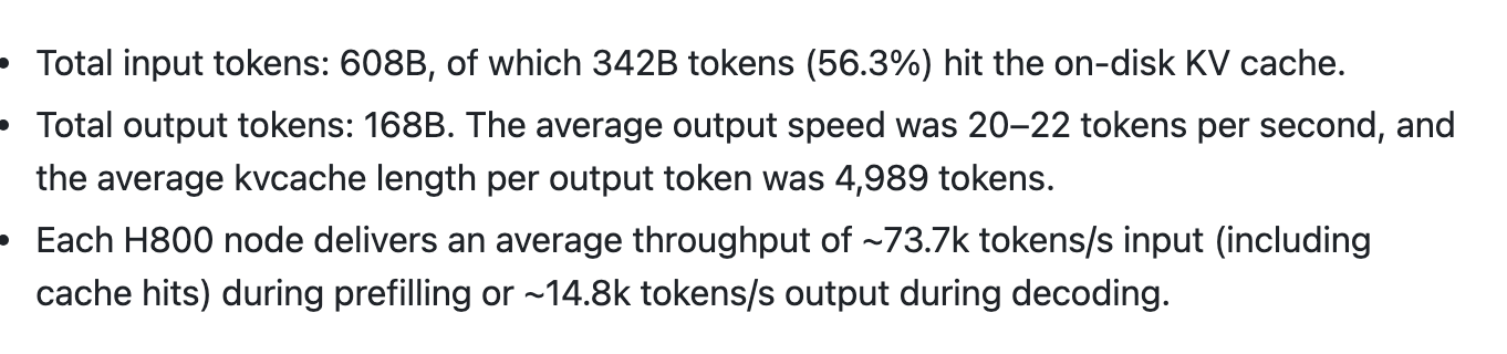
Each H800 node delivered about 73.7 thousand input tokens per second in prefill (including cache hits) or about 14.8 thousand output tokens per second in decode. Prefill nodes move five times more tokens, which is the compute-bound against memory-bound gap of Part 1 showing up at cluster scale, and one more reason to give the two phases different machines.
7. Disaggregated prefill and decode
Why the two phases get in each other's way
Part 1 showed that prefill and decode are different kinds of work. Prefill processes thousands of prompt tokens at once and is limited by arithmetic (compute-bound). Decode produces one token per sequence per step and is limited by reading memory (memory-bound). Part 3 showed what happens when one GPU does both: a long prompt arriving in the middle of other users' answers either stalls those answers while it is prefilled, or, with chunked prefill, is cut into slices that slow every step a little for longer.
The cost model of the simulator below makes the interference concrete. A user is one of 32 sequences being decoded on an H100 running Llama 3.1 8B when another user's 2,000-token prompt arrives:
With prefill first, the user's stream freezes for the whole 67.8 ms prefill, six normal steps long. With 512-token chunks, four of the user's steps grow from 11.4 ms to 19.3 ms. On a decode-only GPU nothing happens at all.
The papers: Splitwise and DistServe
Two papers in 2024 made the case for splitting the phases onto separate GPUs. Splitwise (Patel et al., Microsoft and the University of Washington) started from production traces and the observation that decode does not need the newest, most compute-heavy GPUs; it reported clusters with "up to 1.4x higher throughput at 20% lower cost". DistServe (Zhong et al., OSDI 2024) framed the goal as goodput, defined in Part 6 (coming soon): the highest request rate at which a target share of requests still meets both the time-to-first-token (TTFT) and time-per-output-token (TPOT) objectives. Its Figure 1 is the clearest picture of the problem:
Notice what the baseline was: "existing systems" in early 2024 meant vLLM without chunked prefill. That matters for our own simulation below.
The cost: moving the KV cache
Splitting the phases adds one job: the prompt's KV cache, built on the prefill GPU, must be copied to the decode GPU before the second token. Its size is the bytes-per-token of Section 1 times the prompt length, and its transfer time is size over bandwidth:
where:
- is the number of prompt tokens and the numerator is the KV cache in bytes (Section 1);
- is the bandwidth of the path between the two GPUs.
DistServe works one example; our script reproduces it first, to check the formula:
Worked example (check). OPT-66B has 64 layers and full multi-head attention with width 9,216, so bytes per token; times 512 tokens is bytes = 1.125 GiB, and at 10 per second, 90 Gibit/s. The paper's 1.13GB and 90Gbps are the same numbers counted in powers of two.
Worked example (today). Llama 3.1 70B, an 8,192-token prompt: GiB. Over one 400 Gb/s card (50 GB/s): 54 ms. Over NVLink in the same server: 6 ms. If the prefill side runs TP=8 and the decode side runs TP=8, each GPU holds one eighth of the cache and can send it over its own network card, so the 8 cards together move it in 6.7 ms.
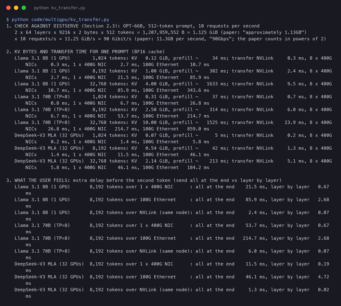
Two things make this cheaper than it looks. First, MLA: DeepSeek-V3's 8,192-token cache is only 0.54 GiB, a fifth of 70B's. Second, the transfer does not have to wait for the prefill to finish. Splitwise sends each layer's KV as soon as that layer is done:
With layer-by-layer sending, what is left after the prefill is roughly the larger of one layer's share and the part of the transfer that did not fit under the computation:
where is the number of layers and the prefill time. For the 70B example over one card: the transfer (54 ms) is far shorter than the prefill (about 314 ms at the assumed efficiency), so only one layer's share is left: ms.
Splitwise measured the effect on real hardware:
Mooncake: build the system around the KV cache
Moonshot AI's Mooncake, the serving platform behind their Kimi assistant, takes the idea one step further. If KV caches are going to travel between machines anyway, treat them as the central object: keep them in a pool spread across the cluster's spare CPU memory and SSDs, and schedule every request by where its cache already is.
DeepSeek's production numbers from Section 6 show the same pattern at scale: 56.3% of their input tokens hit an on-disk KV cache.
A simulation: when is it worth it?
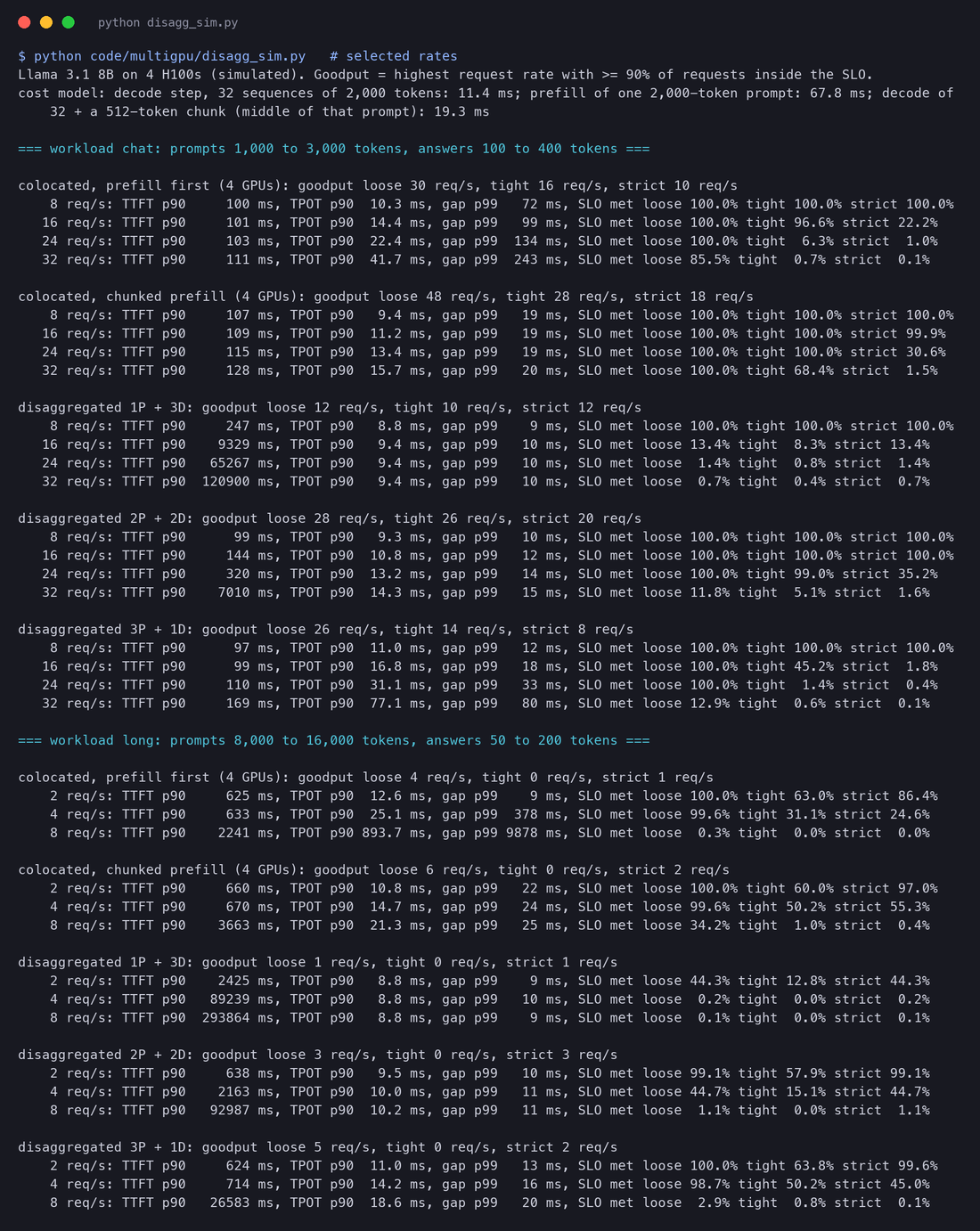
The papers report big wins against the systems of their time. Engines have improved since, especially with chunked prefill. So disagg_sim.py compares the options on equal hardware, under clearly stated assumptions:
- 4 H100s serving Llama 3.1 8B. Each iteration costs ms, with attention FLOPs counted for prompts. The 70% and 50% efficiencies and the 1 ms overhead are assumptions.
- Layouts: four colocated GPUs with prefill first; four colocated GPUs with 512-token chunked prefill; and disaggregated 1+3, 2+2 and 3+1 prefill and decode GPUs, with the KV cache moved over NVLink.
- Workloads: "chat" with 1,000 to 3,000-token prompts and 100 to 400-token answers; "long" with 8,000 to 16,000-token prompts and 50 to 200-token answers. Poisson arrivals for 120 simulated seconds.
- SLOs: loose (TTFT 1 s, TPOT 40 ms), tight (TTFT 0.5 s, TPOT 15 ms) and strict (TTFT 1 s, TPOT 12 ms). Goodput is the highest rate at which 90% of requests meet both.
The heart of the simulator is the cost of one iteration and the three kinds of iteration a GPU can run:
def iter_time(decode_reqs, prefill_tokens, extra_flops=0.0):
    kv = sum(r['ctx'] for r in decode_reqs) * KV_TOK          # every running sequence's cache is read
    toks = len(decode_reqs) + prefill_tokens
    return max((W_BYTES + kv) / HBM, (2 * P * toks + extra_flops) / PEAK) + OVH
A prefill-first GPU runs a whole-prompt iteration whenever prompts are waiting, so everyone decoding waits; a chunked GPU adds up to 512 prompt tokens to every decode iteration; a disaggregated prefill GPU only prefills, then schedules a hand-off event later, when the request joins the least-loaded decode GPU.
| Goodput, requests/s on 4 GPUs (simulated) | Chat, loose | Chat, tight | Chat, strict | Long, loose | Long, strict |
|---|---|---|---|---|---|
| Colocated, prefill first | 30 | 16 | 10 | 4 | 1 |
| Colocated, chunked prefill | 48 | 28 | 18 | 6 | 2 |
| Disaggregated 1P + 3D | 12 | 10 | 12 | 1 | 1 |
| Disaggregated 2P + 2D | 28 | 26 | 20 | 3 | 3 |
| Disaggregated 3P + 1D | 26 | 14 | 8 | 5 | 2 |
(No layout meets the tight SLO on the long workload: a 12,000-token prompt alone takes about half a second to prefill on one GPU.)
What the simulation says, honestly:
- Disaggregation removes the stalls. In the chat workload at 16 requests per second, prefill-first has a 99th-percentile gap between tokens of 99 ms (worst 236 ms); chunked prefill 19 ms; 2P + 2D 12 ms. On long prompts, prefill-first freezes some users for up to 1.4 seconds.
- But on a handful of GPUs, chunked prefill usually wins on goodput. With only 4 GPUs, the split must be 1+3, 2+2 or 3+1, and every ratio wastes some capacity. Chunked prefill uses all four GPUs for whatever work exists. Under the loose and tight SLOs it serves the most requests on both workloads.
- Disaggregation wins when the time-per-token target is strict. Under the strict 12 ms TPOT, 2P + 2D serves 20 chat requests per second against 18, and 3 long-prompt requests against 2, because chunked steps that carry prompt slices are slower than pure decode steps.
- The ratio is everything. The same four GPUs serve 12, 28 or 26 chat requests per second (loose SLO) depending on the split. Production systems pick and adjust the ratio continuously; DistServe searches for it automatically.
The vLLM documentation states the same conclusion in one line:
So disaggregation is worth it when: prompts are long; the per-token latency target is strict; the deployment is large enough to choose the prefill-to-decode ratio finely (DeepSeek runs thousands of GPUs); the two phases benefit from different parallel layouts (DeepSeek's EP32 prefill against EP144 or EP320 decode); and there is fast networking for the KV cache. For one or two servers of a mid-sized dense model, chunked prefill on every GPU is the simpler and often better choice.
8. Real systems today
Everything above is available as flags in the open-source engines. Here is how each idea maps to them, checked against the current documentation (11 October 2026). Flags change between releases, so check the docs for your version.
vLLM
The vLLM docs give the same rule of thumb this article arrived at:
| Idea | vLLM flag | Note |
|---|---|---|
| Tensor parallel | --tensor-parallel-size 8 | Inside one NVLink node |
| Pipeline parallel | --pipeline-parallel-size 2 | Across nodes, with TP inside each |
| Data parallel (copies) | --data-parallel-size 8 | With EP: attention copied, experts spread |
| Expert parallel | --enable-expert-parallel | EP size = TP size x DP size |
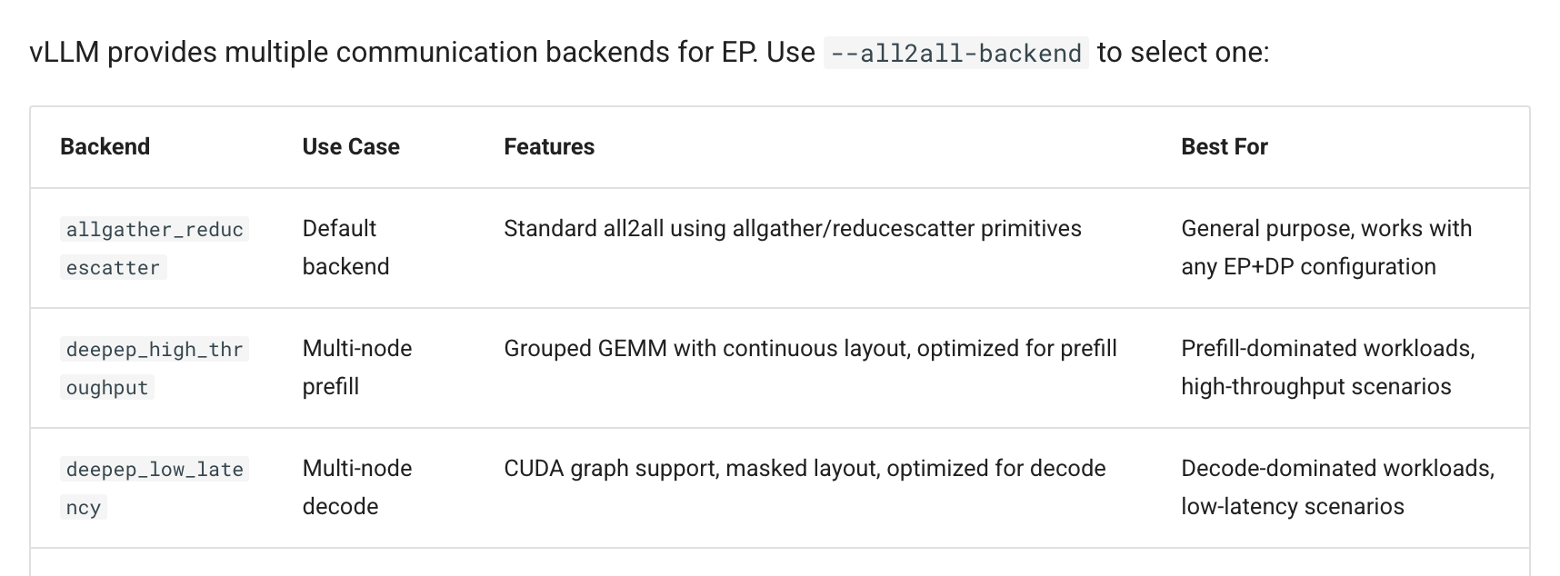
| All-to-all kernels | --all2all-backend deepep_low_latency | Also deepep_high_throughput, allgather_reducescatter (default) |
| Expert load balancing | --enable-eplb, --eplb-config '{...}' | Redundant experts, as in Section 6 |
| Disaggregated prefill | --kv-transfer-config '{"kv_connector":"NixlConnector","kv_role":"kv_both"}' | Connectors include NIXL, Mooncake, LMCache; marked experimental |
Typical launches, from the documentation:
# Llama 3.1 70B on one 8-GPU node
vllm serve meta-llama/Llama-3.1-70B-Instruct --tensor-parallel-size 8

# A model too big for one node: TP inside each of 2 nodes, PP across them (after joining the nodes as the docs describe)
vllm serve <model> --tensor-parallel-size 8 --pipeline-parallel-size 2

# DeepSeek-V3 on one node: attention copied 8 ways, experts spread over 8 GPUs
vllm serve deepseek-ai/DeepSeek-V3-0324 --tensor-parallel-size 1 --data-parallel-size 8 --enable-expert-parallel
The expert-parallel page lists the all-to-all backends, split by the two phases exactly as DeepSeek splits them:
SGLang
| Idea | SGLang flag | Note |
|---|---|---|
| Tensor parallel | --tp-size (or --tensor-parallel-size) | |
| Pipeline parallel | --pp-size | |
| Data parallel copies | --dp-size | |
| Data-parallel attention | --attn-dp-size | Replaces the older --enable-dp-attention, now deprecated |
| Expert parallel | --ep-size | |
| All-to-all kernels | --moe-a2a-backend deepep | Also mooncake, nixl, flashinfer and others |
| Expert load balancing | --enable-eplb | |
| Disaggregation | --disaggregation-mode prefill or decode | Transfer with --disaggregation-transfer-backend mooncake (default) or nixl |
SGLang's PD disaggregation page explains the motivation in the terms of Section 7, including a problem specific to data-parallel attention:
A single-node disaggregated setup from that page (Llama 3.1 8B, one GPU each, Mooncake transfer) is three commands:
python -m sglang.launch_server --model-path meta-llama/Llama-3.1-8B-Instruct \
  --disaggregation-mode prefill --port 30000 --disaggregation-ib-device mlx5_roce0
python -m sglang.launch_server --model-path meta-llama/Llama-3.1-8B-Instruct \
  --disaggregation-mode decode --port 30001 --base-gpu-id 1 --disaggregation-ib-device mlx5_roce0
python -m sglang_router.launch_router --pd-disaggregation \
  --prefill http://127.0.0.1:30000 --decode http://127.0.0.1:30001 --host 0.0.0.0 --port 8000
The router receives each request, sends it to a prefill server, and has the decode server pick up the KV cache over RDMA (the mlx5_roce0 device is the RDMA network card). The page's DeepSeek-V3 example uses two prefill nodes with --tp-size 16 --attn-dp-size 8 --moe-a2a-backend deepep: attention in data-parallel groups, experts over all 16 GPUs with DeepEP.
The orchestration layer: Dynamo and llm-d
Running disaggregation and wide expert parallelism in production needs more than one engine process: routers that know where each KV cache lives, a way to move KV between machines, and autoscaling of the prefill and decode pools separately. Two open-source projects package this around the engines:
- NVIDIA Dynamo describes itself as "the open-source, datacenter-scale inference stack". It runs on top of SGLang, TensorRT-LLM or vLLM ("it doesn't replace" them) and adds disaggregated prefill and decode pools that scale independently, KV-aware routing ("based on worker load and KV cache overlap"), and a KV block manager that offloads cache from GPU to CPU, SSD and remote storage. Its transfer library, NIXL (NVIDIA Inference Xfer Library), is also one of vLLM's KV connectors and SGLang's transfer backends. Latest release at the time of writing: v1.5.1, 7 October 2026.
- llm-d, a Cloud Native Computing Foundation sandbox project started by Red Hat, Google Cloud, IBM Research, CoreWeave and NVIDIA, is "a high-performance distributed inference serving stack optimized for production deployments on Kubernetes". Its documented "well-lit paths" include prefix-cache-aware routing, prefill/decode disaggregation, and "wide expert parallelism" for large MoE models. Latest release: v0.10.0, 29 September 2026.
Both build on vLLM (and in Dynamo's case SGLang and TensorRT-LLM as well); neither replaces the parallelism inside an engine. They decide which engine instance a request goes to and where its KV cache moves, the cluster-level version of the routing in Part 6 (coming soon).
9. Choosing a layout
A decision guide
Worked example 1: Llama 3.1 8B
Weights 16 GB, 128 KiB of KV per token. One H100 holds the model plus tokens of KV cache: 52 conversations of 8,192 tokens. The decode floor is 4.8 ms per step on one GPU. Use one GPU per copy, and add copies for more traffic. Tensor parallelism would only add all-reduces to a model that already fits; at TP=2 the step floor halves to 2.4 ms, which is worth it only if a per-token latency target cannot be met otherwise. Disaggregation, by our simulation, does not raise goodput at this size unless the per-token target is very strict. Everything else about scaling this model is in Part 6 (coming soon).
Worked example 2: Llama 3.1 70B on one 8-GPU node
The weights (141 GB) need at least two GPUs, and realistically more to leave room for KV. With 8 GPUs, three layouts are possible: one copy at TP=8, two copies at TP=4, or four copies at TP=2. The model in layout_model.py compares them for 4,096-token conversations:
| Layout | KV room (4,096-token conversations) | Batch 1: ms per token | Batch 64 per copy: ms per token, node tokens/s | Most the node can do |
|---|---|---|---|---|
| TP=8, 1 copy | 324 | 6.9 | 10.7 ms, 5,969 (batch 128: 14.6 ms, 8,779) | 11,482 tokens/s at 22.3 ms (batch 256) |
| TP=4, 2 copies | 109 each, 218 total | 12.2 | 19.1 ms, 6,702 | 6,702 tokens/s at 19.1 ms (batch 64) |
| TP=2, 4 copies | 2 each | 22.9 | (does not fit) | 347 tokens/s |
Worked numbers for TP=4. Each copy has GB usable; the weights take 141 GB, leaving 147 GB, which at GiB per conversation holds 109 conversations. For TP=8 the free memory is GB: 324 conversations, three times as many, because the weights are stored once instead of twice.
You may have heard "prefer more copies over wider tensor parallelism". For a 70B model on 80 GB GPUs this model says the opposite. At the same 128 sequences in flight on the node, one TP=8 copy makes 8,779 tokens per second at 14.6 ms per token, while two TP=4 copies (64 each) make 6,702 at 19.1 ms. Decode is memory-bound, and two copies read the 141 GB of weights twice per step where one copy reads them once. The extra all-reduces of TP=8 cost less than that second read. TP=8 also has three times the KV room, so it can go on to 11,482 tokens per second at batch 256, and it gives the lowest latency for a single user (6.9 against 12.2 ms). TP=2 barely fits the weights and is useless.
More copies do win in other conditions: when the weights are a small part of each step's memory traffic (long contexts, where the KV cache dominates), when the links are slow (no NVLink, so all-reduce is expensive), and for reasons a roofline ignores, such as isolating failures and scheduling requests independently. So the lesson is a method, not a rule: count the KV room for each layout first, then compare latency and throughput at the batch sizes your traffic needs, and confirm with a benchmark as in Part 6.
Worked example 3: a large MoE across nodes
DeepSeek-V3 in FP8 needs 671 GB for weights: at least nine 80 GB GPUs, so more than one node. Its attention is small and its KV cache tiny (68.6 KiB per token), so copying attention is cheap; its experts are huge, so spreading them is the only option. The layouts from Section 6 follow:
- Small deployment (2 nodes, 16 GPUs): attention in data-parallel groups, experts spread over all 16 GPUs with EP, DeepEP for the all-to-all. This is SGLang's documented two-node example.
- Large deployment (dozens of nodes): separate prefill and decode units, with wider EP for decode (EP144 to EP320 in DeepSeek's case), redundant copies of hot experts, and two micro-batches to hide the all-to-all.
The all-to-all cost from Section 6 sets the limits. At about 11 ms of dispatch and combine per decode step at EP8 (more at wider EP), the communication must be overlapped with computation, and the network matters as much as the GPUs. That is why DeepSeek limits each token to 4 nodes, and why the decode units are so large: many GPUs reading their own experts in parallel is what makes a 37-billion-active-parameter step fast.
10. Summary
The whole part, on one page
| Question | Answer | Where the number comes from |
|---|---|---|
| Why more than one GPU? | 70B needs 227 GB with KV for 32 x 8K conversations; 405B BF16 weights (812 GB) exceed one 8-GPU node | Arithmetic from published shapes |
| What does spreading buy? | Each GPU reads 1/p of the weights: 70B decode floor 21.1 ms on 2 GPUs, 5.3 ms on 8 | Arithmetic, H100 peak bandwidth |
| How fast are the wires? | HBM 3,350, NVLink 900, PCIe 128, one 400G NIC 50 GB/s | NVIDIA spec pages |
| What is a message's cost? | : small messages cost a fixed delay | Measured shape on this laptop; NVIDIA publishes no alpha |
| Tensor parallelism | Columns then rows: 2 all-reduces per layer; exact (same 24 tokens, logits within ) | Measured: 2-process Qwen2.5-0.5B run |
| Its cost | 160 all-reduces per 70B step; 23% of a TP=8 step at batch 1 | Model, assumed 5 s |
| Ring all-reduce | Bytes , but steps; two-step algorithms cut latency 7x at TP=8 | Simulation and formula |
| Pipeline parallelism | Little traffic, no latency gain; with micro-batches 1.7x the throughput of TP=16 across two nodes | Model, 405B |
| Expert parallelism | 10 MB of all-to-all per token for DeepSeek-V3; real routing makes the busiest GPU 1.3x to 6.8x the average | DeepEP report checked by arithmetic; measured OLMoE routing |
| Fixing MoE imbalance | Place by load (1.81 to 1.12 at EP=8 on code); copy hot experts (6.75 to 1.67 at EP=64) | Simulation on measured routing |
| Disaggregation | Moves 2.5 GiB per 8K-token 70B prompt (54 ms on one NIC, under 1 ms exposed layer by layer); wins under strict TPOT and at scale, not by default | Arithmetic; simulation |
Return to where we started. A 70B model does not fit on one GPU, so it is cut into pieces that must talk. Inside a server, where talking is cheap, every layer is split (tensor parallelism) and the GPUs add up their partial results 160 times per token. Between servers, where talking is slow, the model is cut into stages (pipeline parallelism) that pass one message per step. Mixture-of-experts models send each token to the GPUs holding its experts (expert parallelism), and the real difficulty is that some experts are far more popular than others. Finally, the two phases of every request can live on different GPUs (disaggregation), at the price of moving the KV cache, which pays off for long prompts, strict per-token targets and large fleets. In every case the design follows one question: how often must the GPUs talk, and how fast is the wire?
The series so far
| Part | Topic | The one idea |
|---|---|---|
| 1 | Prefill and decode | Decode is limited by reading the weights, not by arithmetic |
| 2 | The KV cache | Saving keys and values avoids recomputation, and their size limits the batch |
| 3 | vLLM | Paged memory, continuous batching and chunked prefill keep one GPU busy |
| 4 | Speculative decoding | Checking several guessed tokens costs about as much as writing one |
| 5 | SGLang and vLLM | Reuse the saved state of shared prompt beginnings |
| 6 (coming soon) | Serving in production | Measure goodput against SLOs, plan capacity, route between copies |
| 7 | Beyond one GPU | Split the model where the wires are fast; the cost of talking decides the layout |
Try it yourself
All the code is in code/multigpu. Nothing needs an NVIDIA GPU.
python code/multigpu/memory_math.py     # Section 1: memory and the decode floor
python code/multigpu/tp_demo.py         # Section 3: split MLP, 2-process Qwen2.5-0.5B, all-reduce timings
python code/multigpu/measure_mps.py     # Section 3: shard timings (needs an Apple GPU; edit dev for CUDA)
python code/multigpu/collectives.py     # Section 4: ring trace, collectives, cost tables, MoE bytes
python code/multigpu/layout_model.py    # Sections 3, 5 and 9: layouts for 70B and 405B
python code/multigpu/moe_routing.py     # Section 6: records OLMoE routing (14 GB download), then simulates EP
python code/multigpu/kv_transfer.py     # Section 7: KV transfer arithmetic
python code/multigpu/disagg_sim.py      # Section 7: colocated vs disaggregated goodput
If you have a machine with two or more NVIDIA GPUs, change the backend in tp_demo.py from gloo to nccl and put each rank's tensors on cuda:<rank>; the same code then runs real tensor parallelism over NVLink or PCIe, and the all-reduce timings in part C become your own and .
References
Papers
- M. Shoeybi et al. Megatron-LM: Training Multi-Billion Parameter Language Models Using Model Parallelism. arXiv 1909.08053, 2019.
- Y. Huang et al. GPipe: Efficient Training of Giant Neural Networks using Pipeline Parallelism. NeurIPS 2019.
- R. Pope et al. Efficiently Scaling Transformer Inference. MLSys 2023.
- Llama Team, AI @ Meta. The Llama 3 Herd of Models. 2024. Section 6, Inference.
- DeepSeek-AI. DeepSeek-V3 Technical Report. 2024. Sections 3.2.2 and 3.4.
- N. Shazeer et al. Outrageously Large Neural Networks: The Sparsely-Gated Mixture-of-Experts Layer. ICLR 2017.
- D. Lepikhin et al. GShard: Scaling Giant Models with Conditional Computation and Automatic Sharding. 2020.
- P. Patel et al. Splitwise: Efficient Generative LLM Inference Using Phase Splitting. ISCA 2024.
- Y. Zhong et al. DistServe: Disaggregating Prefill and Decoding for Goodput-optimized Large Language Model Serving. OSDI 2024.
- R. Qin et al. Mooncake: A KVCache-centric Disaggregated Architecture for LLM Serving. 2024.
- A. Agrawal et al. SARATHI: Efficient LLM Inference by Piggybacking Decodes with Chunked Prefills. 2023.
- N. Muennighoff et al. OLMoE: Open Mixture-of-Experts Language Models. 2024. The model used in Section 6: OLMoE-1B-7B-0924.
Documentation, specifications and engineering posts
- NVIDIA. H100, H200, NVLink and NVLink Switch, DGX H100 user guide, InfiniBand adapters (ConnectX-7).
- NVIDIA. 3x Faster AllReduce with NVSwitch and TensorRT-LLM MultiShot. Technical blog, November 2024.
- NVIDIA. nccl-tests performance notes (algorithm and bus bandwidth).
- vLLM. Parallelism and Scaling, Expert Parallel Deployment, Disaggregated Prefilling.
- SGLang. Server Arguments, PD Disaggregation.
- DeepSeek. DeepEP (performance tables in the v1.2.1 README); DeepSeek-V3/R1 inference system overview, February 2025.
- NVIDIA Dynamo and documentation; llm-d and its well-lit paths.
Companion results