Serving LLMs in Production: Latency, Capacity, Cost, and What Breaks
TTFT, goodput and honest benchmarks; queueing maths and capacity planning for an 8B model on an H100; cost per million tokens; quantization measured on a real model; routing, multi-LoRA, autoscaling and the failures to watch for.
Parts 1 to 5 built an inference engine from the inside: why decode is slow (Part 1), what the KV cache costs (Part 2), how vLLM pages and batches it (Part 3), how speculative decoding writes several tokens per step (Part 4), and how SGLang and vLLM reuse a shared prompt (Part 5).
Now suppose the engine works, and your team is about to put a model behind an API for the whole company. Different questions take over:
"Is it fast?"                 Fast for whom? The first word, every word, or the whole answer?
"How many GPUs do we need?"   For how much traffic, and how slow is too slow?
"What does a token cost?"     Which token? Reading the prompt and writing the answer cost different amounts.
"Can we make it cheaper?"     Smaller numbers inside the model, fewer copies of it, fewer idle GPUs.
"What will go wrong?"         Usually not the model. Queues, retries, memory, and the one user who sends a novel.
This part answers them in order, with one rule from the earlier parts kept strictly: every number has a source, and you can rerun it.
- What "fast" means: the four latency numbers, percentiles, SLOs, and goodput.
- Benchmarking honestly: closed and open loops, bursts, and the mistake called coordinated omission.
- Queueing maths: Little's law and why waiting explodes near full load, then a simulator of a batching engine.
- Capacity planning on paper: from model size, KV bytes and traffic to a number of H100s.
- Cost per million tokens: why output costs more than input, and why cached input costs less.
- Quantization: INT8, INT4, FP8 and an FP8 KV cache, measured on a real model.
- Routing across replicas: load against cache hits, simulated with SGLang's router rule.
- Multi-LoRA serving: many fine-tunes on one base model, with a real measurement.
- Autoscaling and cold starts: measured load times, and what to scale on.
- What breaks in production: retry storms, preemption storms, long prompts, noisy neighbours, and the metrics to watch.
1. What "fast" means
A chat answer streams in. The user sees nothing for a moment, then the first word, then a steady flow of words, then the end. Each of those moments has its own number, and they measure different parts of the engine.
Rearranged, the three are tied together:
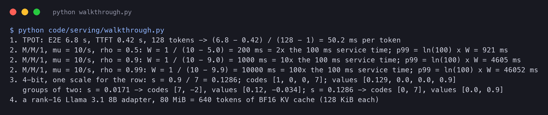
where E2E is what a non-streaming user waits for. A worked example: a request whose first token arrives after 0.42 s and whose 128th and last token arrives after 6.8 s has ms. That is about 20 tokens per second, faster than anyone reads, so this user would complain about the 0.42 s before anything else.
The engines measure exactly these. vLLM's Prometheus endpoint exports them as histograms:
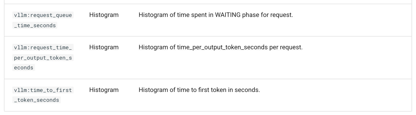

SGLang exports the same four under the names sglang:time_to_first_token_seconds, sglang:inter_token_latency_seconds, sglang:request_time_per_output_token_seconds and sglang:e2e_request_latency_seconds (read in its metrics_collector.py and its production metrics page). Server-side numbers start when the request reaches the server; a user also waits for the network, TLS, your API gateway and any queue in front of the engine. Measure at the client too.
Percentiles, because averages lie
A latency is a distribution, not a number. Here is the TTFT of 3,600 requests from the simulated engine of Section 3, running at a steady 6 requests per second:
The mean (115 ms) sits above the median (93 ms) because a few slow requests pull it up, and it says nothing about the p99 (401 ms), more than four times the median. Two servers with the same mean can have very different tails. Report p50 and p99 (and p99.9 when traffic is large) for each of TTFT, ITL and E2E. Never average percentiles across servers or time windows either: the p99 of two halves is not the mean of their p99s. Prometheus histograms keep the bucket counts precisely so that percentiles can be computed after adding the counts.
SLOs and goodput
A server can be very busy and still useless: if every request finishes, but late, its throughput is high and its users are unhappy. The DistServe paper gave a name to the number that matters.
2. Benchmarking honestly
Every number in Section 1 depends on the load the server was under. So the first question about any benchmark chart is: how was the load generated? Two designs give very different answers on the same server.
A closed loop has a built-in brake. When the server slows down, its users send less, so the server never sees the overload that would happen in production. A closed loop with users can never offer more than requests per second, whatever rate you hoped to test. It is the right model for one batch job with a fixed number of workers, and the wrong one for a public API.
vllm bench serve generates open-loop traffic this way. Its --burstiness option keeps the same average rate but makes the traffic clumpier:

Same mean, different tails. On the simulated engine (Section 3, with its SLO of TTFT ≤ 1 s and TPOT ≤ 50 ms), at the same 5 requests per second:
| Arrivals at 5 requests/s | TTFT p50 | TTFT p99 | Requests inside the SLO |
|---|---|---|---|
| Poisson (burstiness 1.0) | 86 ms | 374 ms | 91.2% |
| burstiness 0.5 | 107 ms | 476 ms | 89.6% |
| burstiness 0.25 | 140 ms | 579 ms | 85.6% |
The average rates are identical; only the clumping changed, and the TTFT p99 grew by more than half. If your real traffic arrives in bursts (a batch job at the top of each hour, a mobile app's morning peak), benchmark with bursts.
Coordinated omission
There is a subtler trap in closed loops, named by Gil Tene in the documentation of his load generator wrk2.
To see it, I simulated the same server (short answers, 5 requests per second) under four measurement methods, and froze the engine for 6 seconds at the 2-minute mark: a GPU hiccup, a long garbage-collection pause, a host problem.
- Open loop, no stall: the baseline.
- Closed loop, as recorded: 10 users, each wanting one request every 2 s, timing each request from the moment it was actually sent.
- Closed loop, from the intended send time: the same run, but each latency measured from when the user wanted to send (wrk2's correction).
- Open loop: Poisson arrivals at 5 per second, with the stall.
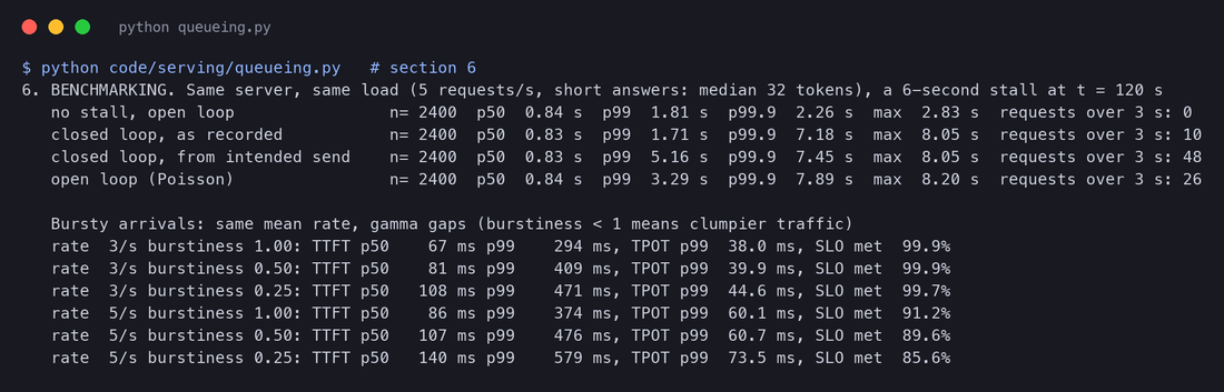
The closed loop as recorded says the p99 is 1.71 s, no worse than a server that never stalled (1.81 s). It saw only 10 slow requests, one per user, because each user stopped sending during the stall. Real users keep arriving: the open loop counted 26 requests over 3 seconds and a p99 of 3.29 s. Measured from the intended send times, the closed loop shows the damage too, and more (p99 5.16 s), because its users fell behind schedule and took time to catch up.
A checklist for a benchmark you can trust
- Open loop at fixed rates, swept from low to past saturation (
vllm bench serve --request-rate), plus a burstier run. Report the rate where the SLO breaks, not only the peak throughput. - Realistic lengths. Prompt and output lengths should follow your traffic, not one fixed pair. Long answers dominate cost (Section 5) and long prompts dominate stalls (Section 10). Make sure the server really generates the lengths you asked for, or your "1,000-token outputs" may stop at the first end-of-text token.
- Warm up (
--num-warmups) and state the cache state. The first requests pay for kernel compilation and an empty prefix cache (Part 5). Then decide whether your real traffic shares prefixes, and test that. - Percentiles of TTFT, ITL and E2E (
--percentile-metrics ttft,tpot,itl,e2el --metric-percentiles 50,90,99), and goodput against your SLO (--goodput ttft:1000 tpot:50, values in ms). - Everything that changes the result: engine version and flags, GPU, model and quantization, request lengths, arrival process, client location.
And what misleading charts look like: throughput without latency ("50,000 tokens per second", at what p99?); latency at one convenient load; a closed-loop "concurrency" axis presented as user traffic; averages instead of percentiles; and a comparison of two engines run with different output lengths or cache states.

3. Queueing maths: why latency explodes near full load
Every serving system is a queue: requests arrive, wait, get served, and leave. Two pieces of queueing theory explain most of what you will see on a latency chart, and both fit on one line.
Little's law
where:
- is the average number of requests in the system (waiting plus being served);
- is the average arrival rate (requests per second);
- is the average time a request spends in the system (for us, the mean end-to-end latency).
It holds for any stable system, whatever the arrival pattern, the scheduling order or the batching. It is how you turn a traffic estimate into memory: requests in flight are what hold KV cache. A worked example: at 10 requests per second and 8 seconds per request, 80 requests are in flight at any moment, each holding its prompt and its answer so far in GPU memory.
To check it, I ran the batching engine simulator (introduced below) at three rates and measured the time-averaged number of requests present directly:
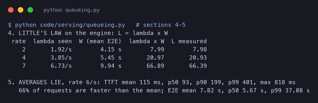
Within 1% at every rate. Notice also how grows faster than the rate: 3.5 times the traffic (2 to 7 per second) put 8.3 times as many requests in flight, because each one also took longer.
Utilisation, and the M/M/1 queue
Take the simplest possible server: one request at a time, random arrivals (Poisson, rate ), random service times (exponential, average ). This is the M/M/1 queue, and its average time in the system is
where is the service rate (requests per second the server could finish if always busy), the average service time, and the utilisation, the fraction of time the server is busy. In this model the time in the system is exponentially distributed, so its p99 is .
The term is the whole story. A worked example with a 100 ms service time ( per second): at 50% utilisation a request takes ms on average, twice its service time. At 90% it takes s, ten times. At 99%, 10 s, a hundred times, with a p99 of 46 s. The last 10% of utilisation costs more than the first 90%.
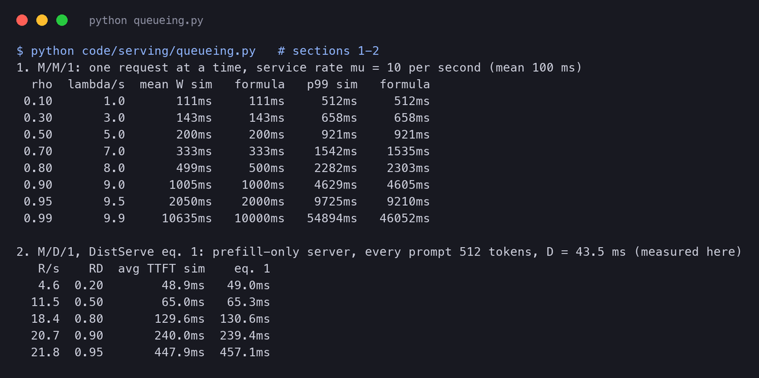
The simulation of 2 million requests per point follows the formula closely up to 90%. At 95% and 99% it is still a little off, which is the same lesson from another angle: so close to full load, the queue swings so widely that even millions of requests are a short sample.
Why does waiting explode? Because arrivals are random. Even when the server is idle 10% of the time on average, it is idle in scattered moments it cannot save up, while bursts of arrivals pile up. Each burst takes longer to clear when there is little spare capacity to clear it with.
The same idea in a real paper: prefill as M/D/1
DistServe uses exactly this reasoning for a server that only does prefill, where every prompt takes the same time (the "D" is for deterministic):
With the laptop's measured time for a 512-token prefill, ms, the simulation matches equation 1 within 2% from 20% to 95% utilisation. At 90% ( per second) a prefill that takes 43.5 ms gives an average TTFT of 240 ms, more than five times as long.
A batching engine is a different kind of server
An LLM engine is not one-at-a-time. With continuous batching (Part 3) it serves many requests together, and the batch grows with the load. To see what that does, I wrote a small discrete-event model of an engine, engine.py, about 250 lines. It follows the main loop of vLLM's scheduler:
decoding = [r for r in self.running if r.done_prefill >= r.need]      # 1. every running request decodes one token
while decoding and self.kv_used() + len(decoding) > self.kv_capacity:  # 2. out of KV memory: preempt the newest
    victim = max(self.running, key=lambda r: r.arrival)
    ...
left = self.budget - len(decoding)                                     # 3. the rest of the token budget goes to
for r in partial_prefills + waiting_requests:                          #    prefill, oldest first, in chunks
    ...                                                                #    (chunked prefill), while memory allows
dt = self.cost(new_tokens, prefill_pairs, kv_tokens_read)              # 4. the step's time from a cost model
Block by block. (1) Requests that have finished their prefill each produce one token per step. (2) If the KV cache cannot hold one more token for each of them, the newest request is evicted and will be recomputed later (Section 10). (3) Whatever is left of the per-step token budget (2,048 here, vLLM's default on smaller GPUs) goes to prompt processing, in chunks, oldest request first; new requests join the batch while memory allows. (4) The step takes as long as the cost model says, and then the clock moves on.
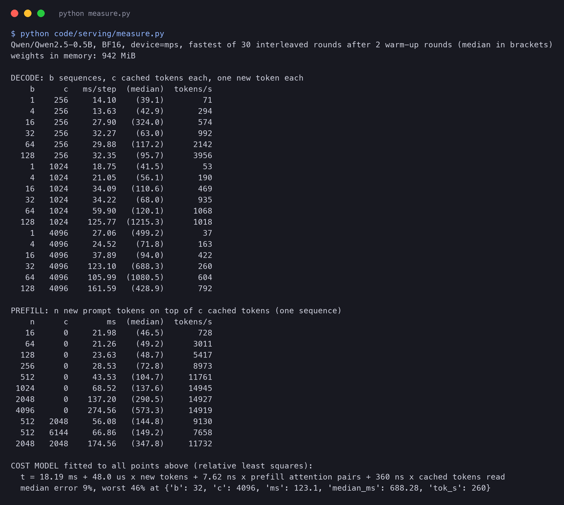
The cost model is fitted to real measurements. measure.py timed Qwen2.5-0.5B on the laptop GPU for 18 decode steps (batch 1 to 128, contexts of 256 to 4,096 tokens) and 11 prefills (16 to 4,096 new tokens, some on top of a cached context), each the fastest of 30 rounds in which every configuration was timed once (so that each had the same chances to catch the shared GPU at a quiet moment), and fitted
where is the number of tokens computed in the step, the number of prefill attention pairs (each new prompt token attends to every earlier token), and the number of cached tokens read (decode reads every sequence's whole KV cache). The fit gives ms, s per new token, ns per prefill pair and ns per cached token read, with a median error of 9% and a worst error of 46% across the 29 measurements. The worst point is a decode step with batch 32 at 4,096 tokens, which measured slower (123 ms) than batch 64 at the same length (106 ms), so the shared GPU clearly disturbed it; the fit is good enough to show shapes and orders of magnitude on this machine, and no better.
Then I offered it Poisson traffic at 1 to 24 requests per second, with prompts around 512 tokens and answers around 128 (lognormal, so some are much longer), 4,000 requests per rate. The SLO, chosen for this small model: TTFT ≤ 1 s and TPOT ≤ 50 ms.
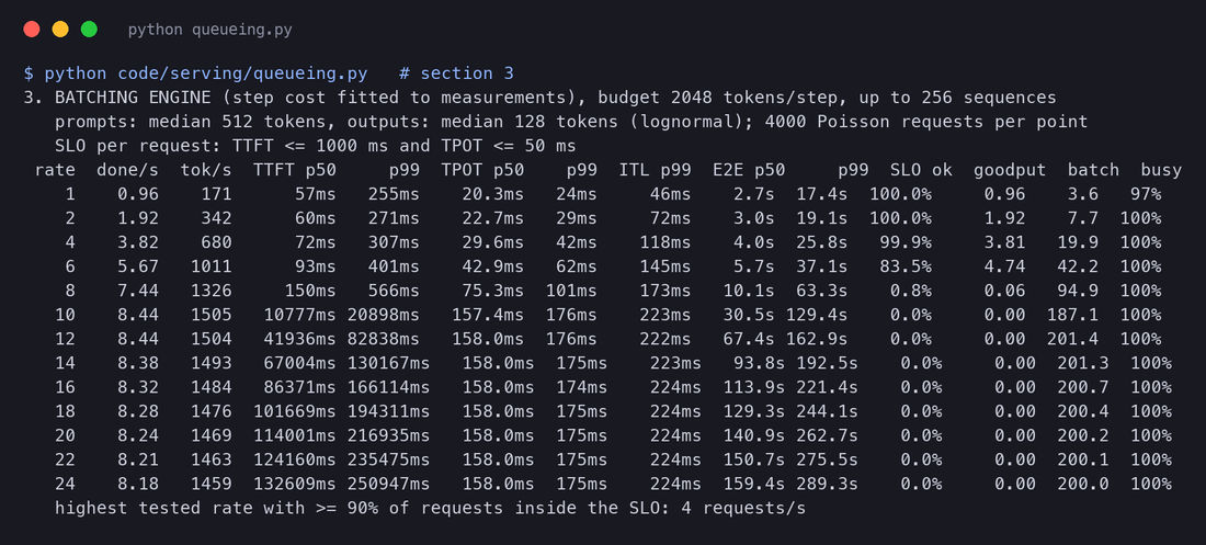
Two things happen, at two different loads.
- TPOT rises steadily (median) from 20 ms at 1 request per second to 75 ms at 8. More traffic means a bigger batch (3.6 sequences on average at 1 per second, 95 at 8), and each step must read every sequence's KV cache, so steps get slower. This is the latency-for-throughput trade from Part 1, now driven by traffic instead of chosen. Its p99 crosses the 50 ms SLO first, between 4 and 6 requests per second.
- TTFT explodes past about 8 per second. Here the engine cannot finish requests as fast as they arrive (it tops out at 8.4 completed requests per second), and the queue grows without bound: p50 TTFT of 150 ms at 8 per second, 10.8 s at 10, 86 s at 16. That is the cliff again, now for a batching server.
Past saturation the server is fully busy finishing requests that have already missed the SLO, so goodput drops to zero while throughput stays at its maximum. A dashboard that shows only throughput would say this server is doing its best work at 24 requests per second. With 99% of requests inside the SLO as the goal, its capacity is about 4 requests per second (99.9% at 4, 83.5% at 6, 0.8% at 8). Half of the throughput that the hardware can deliver is unusable under this SLO.
One more column deserves attention: busy. The simulated GPU was busy 97% of the time at 1 request per second and 100% from 2 per second on. A batching engine always has something to do (decoding whoever is in the batch), so "GPU utilisation" says almost nothing about how much more load it can take. Remember this in Section 9.
4. Capacity planning on paper
Section 3 found the capacity of one small model on one laptop by simulation. Before you buy or rent GPUs for a real service, you want the same answer for a real model on a real data-centre GPU, and you want it before any benchmark exists. This section does it on paper for Llama 3.1 8B on one NVIDIA H100 (80 GB), using only published numbers and stated assumptions. Then it checks the paper answer with the same simulator, driven by the H100's limits instead of the laptop's.
Everything here comes from capacity.py. The inputs are the model's configuration (32 layers, 8 KV heads of 128 numbers, 8.03 billion parameters), the H100 datasheet (989 TFLOP/s of dense BF16 arithmetic, 3.35 TB/s of memory bandwidth) and vLLM's default memory setting. Three inputs are assumptions, marked as such: the traffic, a memory reserve for activations, and later a GPU price.
Step 1: what fits in memory
The GPU's memory holds three things: the weights, some working memory for activations and the runtime, and the KV cache. Whatever is left after the first two becomes KV cache, and the KV cache decides how many requests can be in flight (Part 2, Part 3).
where:
- is the GPU's memory, 80 GB;
- is the fraction the engine may use; vLLM's
--gpu-memory-utilizationdefaults to 0.92 (read invllm/config/cache.py); - is the number of parameters, 8.03 billion, and the bytes per weight (2 for BF16);
- is memory for activations, CUDA graphs and the runtime. vLLM measures this when it starts; here I assume 4 GB;
- is the KV cache per token: bytes, the 128 KiB from Part 2 and Part 5.
With numbers:
util = 0.92                                     # vLLM's default --gpu-memory-utilization
reserve = 4e9                                   # ASSUMPTION: activations, CUDA graphs, CUDA context
weights_bf16 = M['params'] * 2
kv_space = H100['mem_bytes'] * util - weights_bf16 - reserve
tokens_bf16 = kv_space / M['kv_bytes_per_token_bf16']About 408,000 tokens. At an average of 1,125 tokens per request in flight (a 1,000-token prompt plus half of a 250-token answer), that is room for about 360 requests at once. FP8 weights and an FP8 KV cache (Section 6) raise it to about 939,000 tokens.
Step 2: how much traffic, and how much is in flight
Now the assumed traffic: at the busiest hour, 100 requests per second, with prompts of 1,000 tokens and answers of 250 tokens on average. Little's law (Section 3) turns that into the number of requests in flight. If a request takes (another assumption: about 0.5 s to the first token and 30 ms per token after it), then
and their KV cache needs
One H100 has 53.5 GB of KV space. Memory alone says at least three GPUs: .
Step 3: how much arithmetic, and how much reading
Memory is one wall. Time is the other. From Part 1: prefill is limited by arithmetic, decode by reading memory. Each has a simple bound.
Prefill. Every prompt token is multiplied by every weight once, two operations (multiply and add) per weight:
where is the number of weights multiplied per token (7.50 billion; the input embedding is a table lookup, not a multiplication) and is the GPU's peak arithmetic rate. 100,000 prompt tokens per second therefore need GPU-seconds every second: prefill alone needs at least 1.52 GPUs, at 100% of peak, which no real kernel reaches.
Decode. One decode step reads all the weights once, plus the whole KV cache of every sequence in the batch, and makes one token per sequence:
where is the batch size (sequences decoding together), their average context length in tokens, the KV bytes per token, and BW the memory bandwidth (3.35 TB/s). For and :
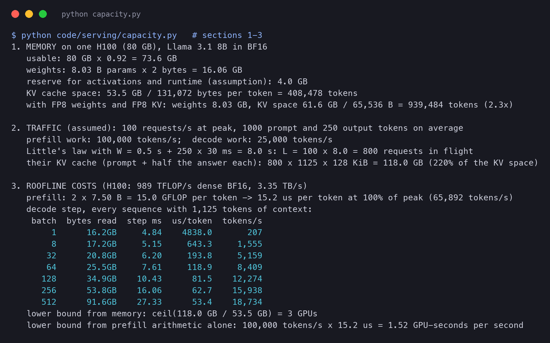
Two lessons sit in this picture. First, batching is what makes decode affordable: from 4,838 µs per token alone to 119 µs at batch 64. Second, even a huge batch cannot make a generated token as cheap as a prompt token, because each sequence's own KV cache must be read at every step. Keep that ratio in mind for Section 5.
Step 4: check it with the simulator
Bounds tell you what is impossible. To find what is possible inside an SLO you need the queueing behaviour from Section 3. So I drove the simulator with the H100 bound instead of the laptop's measured costs: every step takes for exactly the tokens it schedules, with vLLM's H100 defaults of an 8,192-token budget per step and up to 1,024 sequences (read in vllm/engine/arg_utils.py), and the KV memory from Step 1. Requests have lognormal lengths around the assumed means (1,106 prompt and 274 output tokens on average in the sample). The SLO is TTFT ≤ 500 ms and TPOT ≤ 50 ms, and a rate counts as sustainable when 99% of requests meet it.
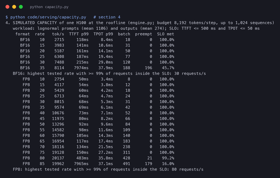
Look at the shape: 100% at 30 requests per second, 45.7% at 35. Between those two points the server stops keeping up: the queue grows, the KV cache fills with requests in progress, the engine starts preempting (196 times in this run; Section 10), recomputation adds work, and the queue grows without limit. In BF16 one H100 sustains at most 30 requests per second of this traffic. FP8 weights and KV (Section 6) halve the bytes per step and double the KV space, and the same GPU sustains 80.
Step 5: the number of GPUs
where is the peak traffic (100 requests per second), the highest rate one GPU sustains inside the SLO (30 from Step 4), the fraction of that you plan to use, and the replicas you keep so that losing one does not break the SLO.
Why plan below 100%? Because came from a roofline, which real kernels never reach, from one traffic mix, and from Poisson arrivals, while Section 2 showed that burstier traffic needs more room. A target of 70% is a common starting point, not a law; your own benchmark decides.
With FP8, . One quantization decision halves the hardware. The three walls also agree with each other: memory said at least 3, prefill arithmetic at least 2, and the queueing check at least 4 at full use.

5. Cost per million tokens
API price lists quote dollars per million tokens, usually with three different prices: input tokens, cached input tokens, and output tokens, with output the most expensive. Section 4 already contains everything needed to see where those prices come from.
A GPU costs money per hour whether it is busy or not. A token costs whatever share of GPU time it used:
where:
- is the price of one GPU for one hour, in dollars. Prices vary by provider, contract and month, so here it is an assumption, shown at $2, $3 and $4 per hour; the cost scales linearly with whatever you pay;
- is the GPU time one token takes, in seconds;
- is the average utilisation: the fraction of the hours you pay for that the GPU spends doing useful work.
Prompt tokens versus generated tokens
Take the BF16 operating point from Section 4 (30 requests per second on one H100, at the roofline). The simulator records how much work each step did. Splitting the GPU's busy time into prefill and decode:
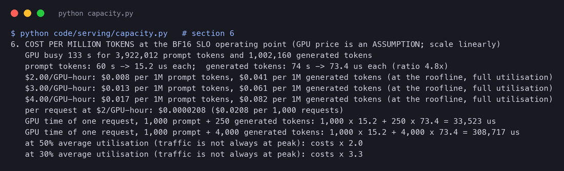
A prompt token costs 15.2 µs and a generated token 73.4 µs: 4.8 times more. This is Part 1's measurement on a laptop (reading 512 tokens took 27 ms, writing 512 took 5.2 s) showing up as a price. Prefill uses the GPU's arithmetic at full efficiency; decode spends most of each step moving bytes.
With $2 per GPU-hour, :
These are floor prices: 100% busy, perfect kernels. Two divisions bring them closer to reality. Divide by the engine's real efficiency against the roofline (your benchmark tells you this). Divide again by the average utilisation: traffic has peaks and valleys, and you provisioned for the peak (Section 4 planned for 70% of capacity at the busiest hour, so the average across a day is lower still). At 30% average utilisation, every price above is 3.3 times higher.
Cached input: why it is cheaper still
A cached prompt token is one whose KV cache already exists (prefix caching, Part 3 and Part 5). Its prefill arithmetic is skipped entirely. Part 5 measured this on the laptop: with an 8,192-token cached prefix, prefill took 22.3 ms instead of 462.3 ms. What a cached token still costs is memory: its KV cache occupies GPU memory while it waits to be reused, and new tokens still read it during attention. That is why providers can sell cached input well below fresh input, and why the discount usually comes with conditions such as a minimum prefix length or a limited lifetime. The arithmetic you skip is free; the memory you hold is not.
Requests, not tokens
Users do not buy tokens; they make requests. Dividing the hourly price by the requests the simulated GPU completed gives $0.0000208 per request at $2 per hour, about 2 cents per 1,000 requests at the floor. Per request, the two kinds of tokens add up separately. With 1,000 prompt tokens, a 250-token answer uses of GPU time; a 4,000-token answer uses , about 9 times more (the script uses the unrounded per-token costs). A request with a 10,000-token document and a short answer is the opposite: mostly prefill. When you estimate the bill for a feature, multiply its expected prompt and answer lengths by these two per-token costs separately; averaging them hides a factor of five.
6. Quantization: a cost lever with a quality price
Section 4 ended with one decision that halved the hardware: storing the weights and the KV cache in 8 bits instead of 16. That decision is called quantization. This section explains what it does to the numbers inside the model, measures what it does to quality on a real model, and is honest about what a laptop cannot show.
Why it speeds up decode follows straight from Part 1: a decode step at a small batch is limited by reading the weights from memory. Halve the bytes, and the step can take about half as long.
Rounding with a scale
The simplest method is round-to-nearest (RTN) with one scale per row of the weight matrix. For -bit signed codes:
where:
- are the original weights in one row (one output channel);
- is the row's scale: the largest weight in the row maps to the largest code ( is 127 for 8 bits, 7 for 4 bits);
- is the stored integer code;
- is the value the model computes with: always a multiple of .
A worked example. Take a row of four weights, , and quantize it to 4 bits. The largest magnitude is 0.90, so . Dividing and rounding gives the codes , and the values the model will use are . Two of the four weights became zero, because one large weight set the scale for the whole row. Split the row into two groups of two and give each group its own scale: the first group has , codes , values , and the small weights survive. That is the whole idea of group quantization: smaller groups, so one large value damages fewer neighbours. The common format "INT4 g128" keeps one scale (and a zero point) for every 128 weights.
def q_int_sym(w, bits, dim=-1):
    qmax = 2 ** (bits - 1) - 1
    s = w.abs().amax(dim=dim, keepdim=True).clamp(min=1e-12) / qmax
return torch.round(w / s).clamp(-qmax - 1, qmax) * sMeasured: what each format does to a real model
I applied each scheme to Qwen2.5-0.5B and measured perplexity on the whole WikiText-2 test set (299,078 tokens, 292 windows of 1,024 tokens). Perplexity is the standard quality check for quantization papers: lower is better, and the BF16 model scores 14.65. Two more checks compare each scheme with the BF16 model token by token on the first 24 windows: the KL divergence between their next-token distributions (0 means identical), and how often both pick the same most likely next token.
The schemes are simulated ("fake quantization"): the weights are rounded to the low-precision grid and turned straight back into floats, so the model computes with exactly the values a low-bit kernel would see. This measures quality exactly. It cannot measure speed: no INT4 or FP8 kernel runs on this laptop. The embedding table (which this model shares with its output layer) stays in BF16 in every scheme, as most deployed formats do.
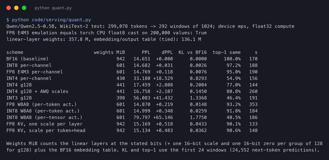
Read the results in four groups.
- 8-bit weights are almost free. INT8 per channel adds 0.03 to perplexity and FP8 adds 0.12. The model still picks the same next token 97% and 95% of the time, and most of the disagreements are between near-equal choices (the KL divergence is 0.003 and 0.008). For memory and bandwidth you get half the bytes.
- 4-bit weights need care. With one scale per row, INT4 more than doubles perplexity (33.2). With groups of 128 it is 17.5, and with AWQ's scales (below) 16.8: usable, but clearly not the same model (77% to 81% top-1 agreement). 3 bits is broken at this size (56.1).
- Activations are harder than weights. Quantizing the inputs of every linear layer too (W8A8) is fine with one scale per token (14.87 for FP8, 15.00 for INT8) and a disaster with one scale for the whole tensor (79.8). The next part explains why.
- An FP8 KV cache costs more than FP8 weights on this model: +0.52 with one scale per layer, and still +0.48 with a separate scale for every token and head.
A small model is the hard case. The papers show larger models losing much less: in AWQ's Table 4, Llama-2-70B goes from 3.32 to 3.46 perplexity with INT4 g128 and plain rounding, a 4% increase, against 19% for our 0.5B model. Measure your own model on your own task before you ship a 4-bit version; perplexity is a first check, not the last.
AWQ: protect the weights that matter
My quant.py implements a simplified version: for each group of layers that read the same input, try for (where is the average magnitude of each input channel on 4,096 tokens of WikiText-2 training text), quantize , and keep the whose outputs best match the original layer. It took INT4 g128 from 17.46 to 16.76, closing a quarter of the gap to BF16, with no extra bits.
Why activations are hard: outliers
Weights are fixed and fairly evenly spread. Activations change with every input, and in large language models a few channels carry values tens of times larger than the rest. One scale for the whole tensor is set by those outliers, and every other value is squeezed onto a handful of codes: that is our 79.8. One scale per token helps because each token's row gets its own range, which is why per-token INT8 and FP8 survived.
The KV cache in FP8
The KV cache can be quantized too: vLLM's --kv-cache-dtype fp8 stores keys and values in 8 bits, which doubles the tokens that fit (Section 4: 408,000 to about 816,000 with BF16 weights) and halves the bytes each decode step reads for attention. On our model it cost more quality than FP8 weights did: +0.52 perplexity with one scale per layer. I expected a finer scale to fix it, so I also tried one scale per token and per head (the idea behind vLLM's newer fp8_per_token_head cache type, listed in vllm/config/cache.py). It helped only a little: +0.48. So the loss here comes mostly from FP8's 3-bit mantissa, a rounding step of up to 1/16 of each value, applied to every key and value of every token, rather than from outliers stretching the range. For a model this small that is a visible price; check it on your own model and task. Note also how vLLM sets the scales: according to its quantized KV cache documentation, with plain kv_cache_dtype="fp8" all scales are 1.0 (no calibration), and the recommended route is to calibrate them on a dataset with the llm-compressor library. My runs used a measured scale for every forward pass, which is kinder than a fixed 1.0. (My rounding happens on the outputs of the key and value projections, before the rotary position encoding is applied; a rotation does not change sizes, so this is a close stand-in.)
What a laptop cannot show
None of these runs measured speed: the rounded weights were turned back into float32 before every multiplication. Real speed-ups need kernels that read the low-bit codes and multiply directly, and they depend on the GPU: weight-only INT4 helps most at small batches (memory-bound), less at large batches where decode becomes compute-bound, and FP8 W8A8 helps prefill too. The capacity simulation in Section 4 is the honest stand-in: on the H100 roofline, FP8 weights plus FP8 KV raised the sustainable rate from 30 to 80 requests per second. The quality numbers above are what you trade for it.
7. Routing across replicas
Section 4 ended with six GPUs. In the simplest deployment each runs its own copy of the model (a replica), and something in front of them, a router or load balancer, decides where each request goes. For ordinary web servers that decision is easy: send it to whoever is least busy. For LLM servers there is a second consideration, and it pulls the other way.
Each replica keeps a prefix cache (Part 5). A request whose system prompt, document or chat history is already cached on replica 2 is much cheaper on replica 2: Part 5 measured a 20.7x faster prefill for an 8,192-token cached prefix. Send it to replica 3 because replica 3 has a slightly shorter queue, and it pays full price, and now two replicas hold the same prefix. So the router must trade load balance against cache affinity.
The policies
| Policy | Rule | Knows about load | Knows about the cache |
|---|---|---|---|
random | pick any replica | no | no |
round_robin | take turns | no | no |
least_outstanding | fewest requests queued or running | yes | no |
power_of_two | sample two, take the less loaded | yes | no |
prefix_hash | hash the prefix, always the same replica (also: session stickiness) | no | yes |
cache_aware | SGLang's router rule, below | yes | yes |
SGLang's router (now called the SGLang Model Gateway) implements the first four and a cache-aware rule, and makes cache-aware the default:
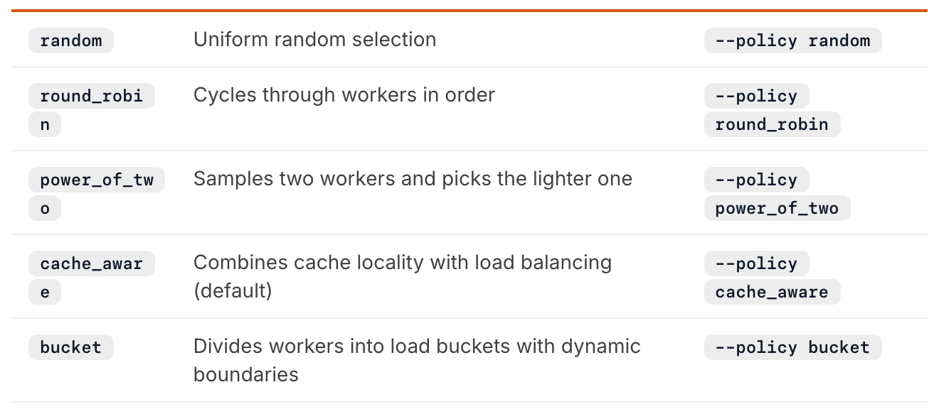
The documentation lists the cache-aware rule's parameters but not the rule itself. The source code does, in a comment at the top of sgl-model-gateway/src/policies/cache_aware.rs:
The router dynamically switches between these strategies based on load conditions:
- Uses load balancing when the system is imbalanced
- Uses cache-aware routing when the system is balanced

A system is considered imbalanced if both conditions are met:
1. (max - min) > abs_threshold
2. max > rel_threshold * min
...
a. For each request, find the worker with the highest prefix match
b. If match rate > cache_threshold:
   Route to the worker with highest match (likely has relevant data cached)
c. If match rate <= cache_threshold:
   Route to the worker with smallest tree size (most available cache capacity)
The router does not ask the replicas what they have cached. It keeps its own approximate radix tree per worker, built from the requests it has sent, over raw text rather than tokens to avoid tokenizing. The defaults:
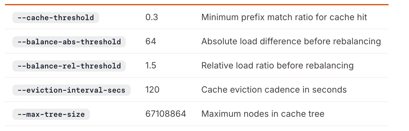
vLLM's Kubernetes deployment, the vLLM Production Stack, has a router with --routing-logic choices roundrobin, session, kvaware, loadaware, prefixaware and two disaggregated-prefill modes (read in its parser.py). llm-d's endpoint picker "scores and selects model server pods based on real-time metrics, KV-cache affinity, and configured policies" (llm-d architecture page). The vocabulary differs; the trade is the same.
Simulated: seven policies, two kinds of traffic
route.py puts four copies of the laptop-calibrated engine behind a router. Every request starts with one of 200 shared prefixes of 2,048 tokens (think: 200 customers, each with a long system prompt and documents), followed by a question of about 128 tokens, and asks for an answer of about 64 tokens. Each replica's prefix cache holds 16 prefixes with least-recently-used eviction, and a hit skips the prefix's prefill. Traffic is 20 requests per second in total, 5 per replica: busy, but within what four replicas can serve. Two popularity patterns:
- Zipf: a few prefixes are popular and there is a long tail (the -th most popular prefix gets traffic proportional to ).
- Hot: one prefix takes 50% of all traffic (one huge customer, or one system prompt shared by everyone), the rest Zipf.
cache_aware implements the rule above with the gateway's defaults; cache_aware (abs 8) is the same rule with --balance-abs-threshold 8.
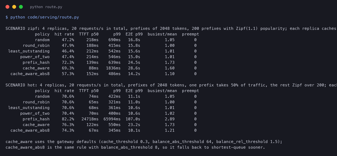
What the simulation shows:
- Load-only policies get the "free" hits only. Random, round robin, least outstanding and power of two all land near 47% hit rate with Zipf traffic: each replica ends up caching the most popular prefixes by itself, and everything else misses. Their TTFT p99 is 415 to 690 ms.
- Pure affinity gets the most hits, and the worst tail when traffic is uneven.
prefix_hashreaches 72% (Zipf) and 82% (hot), because each prefix lives on exactly one replica. But popularity is not balanced: with Zipf the busiest replica got 1.73 times its share of requests, and end-to-end p99 rose from 15.8 s (round robin) to 24.5 s. With one hot prefix, one replica got 2.89 times its share, overloaded, and TTFT p99 went to 66 seconds. Session stickiness has the same weakness when one session or tenant is much bigger than the rest. - Cache-aware routing gets most of the hits without most of the cost, if its balance threshold fits your scale. With the default threshold of 64 outstanding requests,
cache_awarereached 69% hits and by far the best median TTFT (88 ms), but the busiest replica carried 1.60 times its share and TTFT p99 was 1.8 s. On this small engine, 64 requests of imbalance is a lot. With a threshold of 8, it gave up some hits (57%), kept TTFT p99 at 486 ms, and had the lowest end-to-end p99 of all seven (14.2 s). With the hot prefix it matched round robin's tail (TTFT p99 345 ms against 321 ms) with 74% hits instead of 71%, and again the lowest end-to-end p99 (10.1 s).
The general rule: route for cache hits while the replicas are balanced, and fall back to the least-loaded replica as soon as they are not. What counts as "not balanced" depends on how many requests a replica normally runs, so tune the threshold to your batch sizes rather than trusting a default.
8. Many fine-tunes, one base model: multi-LoRA serving
Sooner or later, different teams want their own version of the model: one tuned on support tickets, one on legal text, one for each large customer. Serving each as a separate model multiplies everything in Section 4 by the number of versions. If the versions are LoRA fine-tunes of one base model, they can share almost all of it.
The memory arithmetic
One adapter adds parameters per adapted layer:
where is the rank, the number of transformer blocks, and the sum runs over the projections that carry an adapter in each block. For Llama 3.1 8B with adapters on all seven projections (q, k, v, o: 4,096 in, and 4,096 or 1,024 out; gate and up: 4,096 to 14,336; down: 14,336 to 4,096), the sum per block is 81,920, so
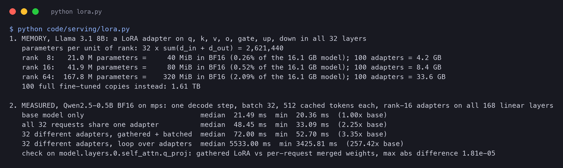
At rank 16 that is 41.9 million parameters, 80 MiB in BF16, 0.52% of the 16.1 GB model. A hundred such adapters take 8.4 GB. A hundred full fine-tuned copies would take 1.61 TB, twenty H100s just to hold them.
The compute problem: a batch of different adapters
Memory is the easy part. The hard part is the batch. Continuous batching (Part 3) mixes requests from many users in every step. If request 1 wants adapter A, request 2 adapter B and request 3 adapter C, the base model's product can still be done as one big matrix multiply for all of them, but each request's correction uses different matrices.
Measured: four ways to run 32 adapters
To see the problem, I ran the same decode step on Qwen2.5-0.5B (BF16, on the laptop GPU) with a batch of 32 requests, each with 512 tokens of context, and rank-16 adapters on all 168 linear layers, in four ways:
def hook(mod, inp, out):                     # runs after every linear layer
    x = inp[0]                               # (batch, tokens, d_in)
    if mode == 'gather':                     # all requests at once: x A[idx] B[idx]
        return out + torch.bmm(torch.bmm(x, A[idx]), B[idx])
    if mode == 'same':                       # every request uses adapter 0
        return out + (x @ A[0]) @ B[0]
    y = out.clone()                          # 'loop': one product per distinct adapter
    for a in idx.unique().tolist():
        rows = (idx == a).nonzero().squeeze(1)
        y[rows] += (x[rows] @ A[a]) @ B[a]
    return y
A stacks all 32 adapters' first matrices, idx says which adapter each request uses, and A[idx] gathers one matrix per request so that a single batched product (bmm) does all 32 corrections. This is the gather idea of Punica and S-LoRA written in plain PyTorch, without their fused kernels.
| How the adapters run | Decode step (fastest of 10) | Against the base model |
|---|---|---|
| Base model, no adapter | 20.4 ms | 1.00x |
| One adapter shared by all 32 requests | 33.1 ms | 1.63x |
| 32 different adapters, gathered and batched | 52.7 ms | 2.59x |
| 32 different adapters, a loop over adapters | 3,425.8 ms | 168x |
Three things to take from it:
- The answer is right. On the first layer, the gathered result matches merging each request's adapter into its own copy of the weights to within (float32 rounding).
- The loop is unusable. One small product per adapter per layer, with a synchronisation to find which rows use which adapter, turns a step into seconds. This is why multi-LoRA serving needed new kernels at all.
- Even the gathered version is not free here. On a 0.5B model the base layers are tiny, so two extra launches per layer (168 layers) cost more than the layers themselves. Fused kernels such as SGMV remove most of that launch cost, and on an 8B model the base work is 16 times larger while the adapter work stays small, so the relative overhead shrinks. When all traffic uses a single adapter, merge it into the weights and pay nothing.
In the engines
vLLM serves LoRA adapters with --enable-lora, and three settings decide the memory split: --max-loras (adapters that can be active in one batch, default 1), --max-lora-rank (default 16), and --max-cpu-loras (adapters kept in CPU memory, ready to swap in). These names and defaults are from vllm/config/lora.py. Requests name their adapter in the model field, and Prometheus reports active adapters through vllm:lora_requests_info. SGLang, whose authors also wrote S-LoRA, supports multi-LoRA batching too.
9. Autoscaling and cold starts
Section 5 showed that idle GPUs make every token more expensive. The usual answer is autoscaling: run fewer replicas at night and more at the peak. For LLMs it has two catches: a new replica takes a long time to become useful, and the usual signal for scaling does not work.
How long does a cold start take?
A new replica must start a process, import its libraries, read the weights from disk or the network, copy them to the GPU, and run a first forward pass (which sets up kernels). I timed each phase for Qwen2.5-0.5B on the laptop, five times, each in a fresh Python process. Separately, I measured the SSD's read speed on a freshly written 2 GiB file with the operating system's cache turned off (macOS F_NOCACHE), because a model file read a second time comes from memory, not disk.
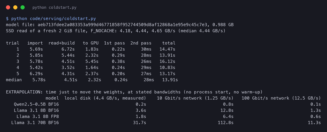
The whole start took 13.9 seconds (median of five) for a model whose weights are under 1 GB: 5.8 s to import PyTorch and Transformers, 4.5 s to read the file and build the model, 2.3 s to copy it to the GPU, and 0.24 s for the first forward pass, against 28 ms for the second. The machine was busy with other jobs, which inflates the CPU-bound phases; still, for a small model, starting the software is most of the cost. The SSD itself delivered 4.4 GB/s, so reading the 0.99 GB file from a cold disk would take about 0.2 s of those 4.5.
For a big model the balance flips. Moving the weights alone, at the measured SSD speed or at typical network speeds (the network speeds are assumptions, labelled as such in the output):
| Model and format | Weights | From local SSD (4.4 GB/s, measured) | 10 Gbit/s network | 100 Gbit/s network |
|---|---|---|---|---|
| Qwen2.5-0.5B, BF16 | 0.99 GB | 0.2 s | 0.8 s | 0.1 s |
| Llama 3.1 8B, BF16 | 16.1 GB | 3.6 s | 12.8 s | 1.3 s |
| Llama 3.1 8B, FP8 | 8.0 GB | 1.8 s | 6.4 s | 0.6 s |
| Llama 3.1 70B, BF16 | 141 GB | 31.7 s | 112.8 s | 11.3 s |
On top of that come container start, engine initialisation, and memory profiling and kernel compilation in engines like vLLM. Minutes are common for large models pulled over a network. During all that time the replica costs money and serves nothing.
What to scale on
The obvious signal, GPU utilisation, is the wrong one. Section 3 found the simulated GPU busy 97% of the time at 1 request per second, an eighth of its saturation rate, because a batching engine is always decoding whoever is in the batch. Scale on signals that measure demand against capacity instead:
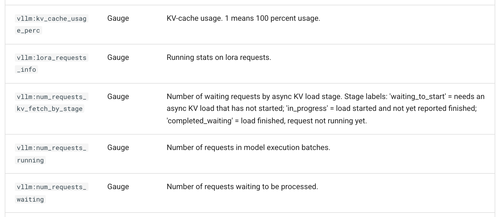
- requests waiting (
vllm:num_requests_waiting,sglang:num_queue_reqs), or requests in flight per replica (waiting plusvllm:num_requests_running); - KV cache usage (
vllm:kv_cache_usage_perc,sglang:token_usage), which rises before the queue does; - the SLO itself: TTFT and TPOT percentiles over the last minutes.
Simulated: a traffic jump, three cold-start times, two signals
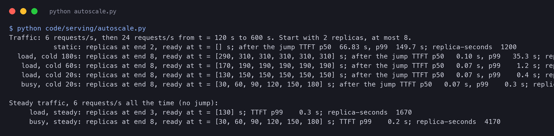
autoscale.py starts with 2 laptop-calibrated replicas at 6 requests per second (3 each: comfortable, since Section 3's engine met the SLO at 4). At s the traffic quadruples to 24 per second, which needs about 6 replicas. Every 10 seconds an autoscaler looks at the replicas that are serving and decides:
- scale on load: target tracking on requests in flight, wanting replicas (20 is about the batch at which Section 3's engine still met the SLO), with cold starts of 180, 60 or 20 seconds, at most 8 replicas;
- scale on GPU busy: add a replica whenever the serving replicas were busy more than 90% of the last interval, with a 20-second cold start.
What it shows:
- The cold start is the latency of your autoscaler. All three load-based runs asked for more replicas at the same moment (130 s). With a 20-second cold start the new replicas served from 150 s, and p99 TTFT over everything after the jump was 0.4 s; with 60 seconds, 1.2 s. With 180 seconds they served from 310 s, and until then users saw what the never-scaling deployment showed, a TTFT p99 climbing past 30 seconds. Over the whole period after the jump, p99 TTFT was 35.3 s, against 149.7 s for never scaling.
- GPU busy is not a load signal. The busy-based policy started adding replicas at 30 s, before the jump, and reached the maximum of 8 by 180 s. With steady traffic of 6 requests per second and no jump at all, it did exactly the same: 8 replicas and 4,170 replica-seconds, where load-based scaling used 1,670 replica-seconds (it added one replica after a burst at 130 s) at a similar p99 (0.3 s against 0.2 s). It only "worked" during the jump because it had already bought everything.
- A backlog makes target tracking overshoot. Ten seconds after the jump, 196 requests were in flight on the two replicas, so the load signal asked for replicas, capped at 8, where the new steady rate needs about 6. Real autoscalers add stabilisation windows and scale down slowly for this reason; scaling down (not simulated here) needs the same care, because a replica that leaves takes its prefix cache with it.
The practical consequences: keep cold starts short (weights on local NVMe or in host memory, images pre-pulled, a warm pool of replicas that have loaded the model and wait without traffic), scale on queue and KV signals rather than utilisation, and plan the base capacity for the jump you cannot react to in time.
10. What breaks in production
Most incidents in LLM serving are not about the model. They are about queues, memory and clients, and they follow a few recognisable patterns. Each one below was reproduced in the simulator (failures.py, laptop-calibrated engine), so you can see its signature before you meet it.
Retry storms: a short hiccup that never ends
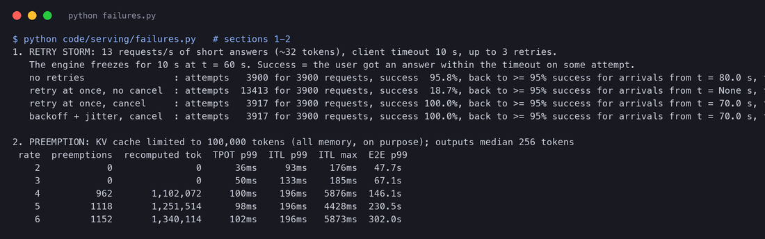
Clients have timeouts, and when a request times out, many clients retry. Picture a healthy server that keeps up comfortably with 13 requests per second of short answers, with a 10-second client timeout and up to 3 retries. At s the engine freezes for 10 seconds. Four combinations of client and server behaviour:
- No retries, no cancellation: requests that arrived just before and during the freeze time out (95.8% success overall). The server still finishes them, generating 5,707 tokens for users who had already left, and recovers for new arrivals 10 seconds after the freeze ended.
- Immediate retries, no cancellation: each timed-out request comes back as a new one, while the server keeps working on the old one. The extra load keeps the queue long, so more requests time out, so more retries arrive. The server never recovers: 13,413 attempts for 3,900 requests, 18.7% success over the run, and 425,460 tokens generated for nobody. The freeze lasted 10 seconds; the outage lasted until the traffic stopped.
- Immediate retries, with cancellation: the server drops a request as soon as its client gives up (the engine's
cancel_on_timeout). Only 17 retries were needed and 100% of users got an answer within the timeout on some attempt. - Backoff and jitter, with cancellation: the same result here, 100%.
This is a metastable failure: a short trigger pushes the system into a bad state that sustains itself after the trigger is gone. The lessons are standard but worth repeating for LLM servers, where each abandoned request may hold memory and generate hundreds of tokens:
- Cancel abandoned work. When the client disconnects or the deadline passes, abort the request in the engine and free its KV cache. Both engines abort a request whose HTTP client has disconnected (vLLM wraps its API handlers with
with_cancellation; SGLang'stokenizer_manager.pychecksrequest.is_disconnected()and callsabort_request). That only helps if every proxy between the user and the engine closes its upstream connection when the user goes away, and if the client's timeout actually closes the connection. - Retry with exponential backoff and jitter, and a retry budget. In this run cancellation alone was enough, because retries were few; when many clients time out at the same moment, spreading their retries out is what keeps them from arriving as a second wave.
- Shed load early. A request rejected at once with "try later" costs nothing; one accepted and abandoned costs its whole prefill and part of its decode.
Preemption storms: when the KV cache is too small
When running requests need more KV cache than exists, vLLM evicts the most recently admitted one and recomputes it later (Part 3); SGLang calls it retraction. A little preemption is harmless. A lot of it is work done twice, and long pauses in the victims' streams. I gave the simulated engine a deliberately small KV cache (100,000 tokens) and longer answers (median 256 tokens):
Up to 3 requests per second: no preemptions, and no stream ever paused for more than 185 ms. At 4 per second: 962 preemptions, 1.1 million tokens computed a second time, and a stream that stopped for 5.9 seconds. At 5 and 6 per second the pattern holds (1,118 and 1,152 preemptions). Like the queueing cliff in Section 3, this one is a switch, not a slope.
What to do: watch vllm:num_preemptions (or sglang:num_retracted_requests_total) and alert on its rate, not its existence; give the KV cache more room (FP8 KV cache, Section 6; a lower --max-num-seqs; fewer LoRA slots; more replicas); and keep --max-model-len no longer than you need, since one maximum-length request can take a large share of the cache.
Long prompts and head-of-line blocking
One user pastes a 16,000-token document while others are chatting. Without chunked prefill, the engine processes that prompt in one step, and every other stream stops while it does. With chunked prefill (Part 3; Sarathi-Serve below), the prompt is cut into pieces that share each step with everyone's decode.

In the simulation, chats at 4 requests per second, and a 16,000-token prompt at s: without chunking the other streams stopped for 1.9 seconds; with a 2,048-token budget the longest pause was 338 ms. The long prompt itself waited a little longer for its first token (2.1 s against 1.9 s), which is the price of fairness.
Noisy neighbours
Shared servers serve several tenants. In the simulation, tenant A sends ordinary chats at 4 requests per second; at s tenant B sends 40 prompts of 6,000 tokens within 10 seconds. With the default first-come, first-served order, tenant A's TTFT for the next 30 seconds went from a p50 of 66 ms to 6.8 seconds, and its p99 from 320 ms to 16.8 seconds. Nothing was wrong with A's requests; they were simply queued behind B's. Defences: per-tenant rate limits at the gateway, per-tenant queues or priorities (vLLM has --scheduling-policy priority; SGLang has --enable-priority-scheduling), separate replicas for very large tenants, and admission limits on prompt length.
The dashboard and the alerts
Every pattern above has a metric. The names below were read in the source code of each engine (vLLM vllm/v1/metrics/loggers.py, SGLang python/sglang/srt/observability/metrics_collector.py).
| Watch | vLLM | SGLang | Alert when |
|---|---|---|---|
| First-token latency | vllm:time_to_first_token_seconds | sglang:time_to_first_token_seconds | p99 above the SLO for several minutes |
| Streaming smoothness | vllm:inter_token_latency_seconds | sglang:inter_token_latency_seconds | p99 above the TPOT SLO |
| Whole request | vllm:e2e_request_latency_seconds | sglang:e2e_request_latency_seconds | p99 drifting up |
| Queue | vllm:num_requests_waiting | sglang:num_queue_reqs | above zero and growing (scale out) |
| Batch | vllm:num_requests_running | sglang:num_running_reqs | near --max-num-seqs |
| KV memory | vllm:kv_cache_usage_perc | sglang:token_usage | above about 90% for long periods |
| Preemption | vllm:num_preemptions | sglang:num_retracted_requests_total | rate rising |
| Prefix cache | vllm:prefix_cache_hits / vllm:prefix_cache_queries | sglang:cache_hit_rate | hit rate dropping after a deploy |
| Time in queue | vllm:request_queue_time_seconds | grows while running stays flat |
Add the outside view: request errors and timeouts at the gateway, client-side TTFT, retries per request, and GPU memory and temperature. Then alert on symptoms users feel (TTFT, errors, timeouts), and use the rest to explain them.
11. Try it yourself
All the code is in code/serving/ of this site's repository. The simulations need only Python's standard library; the measurements need PyTorch and a GPU (or patience on a CPU).
python3 code/serving/walkthrough.py        # the small worked examples
python3 code/serving/queueing.py           # M/M/1, M/D/1, the engine under load, benchmarking traps
python3 code/serving/capacity.py           # the H100 capacity plan and cost per token
python3 code/serving/route.py              # seven routing policies
python3 code/serving/autoscale.py          # cold starts and scaling signals
python3 code/serving/failures.py           # retry storms, preemption, long prompts, noisy neighbours
python3 code/serving/measure.py            # needs torch: step costs for your own GPU (then rerun the above)
python3 code/serving/quant.py              # needs torch: quantization quality on WikiText-2
measure.py writes the cost model that the laptop simulations use. Run it on your own GPU and the queueing, routing and failure experiments recalibrate to your hardware. To check the simulator against a real engine, start vLLM or SGLang with the model you serve and run vllm bench serve with --request-rate swept from low to past saturation, --percentile-metrics ttft,tpot,itl,e2el and --goodput set to your SLO. The shape of Section 3's curves should appear; the numbers will be yours.
The whole part, on one page
| Question | Answer | Where the number comes from |
|---|---|---|
| What is "fast"? | TTFT for responsiveness, ITL and TPOT for streaming, E2E for whole answers, each as p50 and p99 | Definitions; vLLM and SGLang metric names from source |
| What should a benchmark report? | Latency percentiles at open-loop rates up to and past saturation, and goodput against the SLO | A closed loop hid a 6-second stall at p99 (1.71 s against 1.81 s with no stall), simulated |
| Why does latency explode? | Waiting grows as : 10x the service time at 90% utilisation | M/M/1 formula, checked by simulation; DistServe's M/D/1 matched within 2% |
| What limits a batching engine? | TPOT rises with the batch; past saturation the queue grows without bound and goodput falls to zero | Simulated with costs fitted to measured steps: about 4 requests/s with 99% inside the SLO, saturation at 8.4 |
| How many H100s for an 8B model? | Memory, compute and SLO each give a bound; at 100 requests/s: 6 GPUs in BF16, 3 in FP8 (with 70% headroom and a spare) | Published specs and a roofline simulation; upper bounds, to be replaced by a benchmark |
| Why is output pricier than input? | A generated token cost 4.8x a prompt token at the operating point | Roofline simulation; prices per hour are assumptions |
| Is quantization free? | 8-bit weights nearly (+0.03 to +0.12 perplexity); INT4 needs groups and AWQ-style scales (+2.1); activations need per-token scales | Measured on Qwen2.5-0.5B, WikiText-2 |
| How should a router choose? | Prefer the warm replica while loads are balanced, the least loaded when not | Simulated with SGLang's rule: 57% to 74% hits with a tuned threshold, without the hashing tail |
| Can one base model serve many fine-tunes? | Yes: 80 MiB per rank-16 adapter for an 8B model; batched kernels keep mixed batches fast | Arithmetic; measured gather-and-batch against a loop on the laptop |
| What should autoscaling watch? | Queue, in-flight requests and KV use, not GPU busy; cold starts set the reaction time | Measured load phases; simulated scaling |
| What breaks? | Retries without cancellation, preemption storms, unchunked long prompts, noisy tenants | Simulated; each has a metric and an alert |
The series so far
| Part | Question | Main idea |
|---|---|---|
| 1 | Why is generating slow? | Prefill is compute-bound, decode is memory-bound; batching shares each weight read |
| 2 | What does the model remember? | The KV cache: 128 KiB per token for an 8B model, read at every step |
| 3 | How does an engine fit many users? | Paged KV memory, continuous batching, chunked prefill, preemption |
| 4 | Can we write several tokens per step? | A cheap draft, checked in one pass of the big model, with identical output |
| 5 | Can requests share work? | Prefix caching with a radix tree or hashed blocks, and cache-aware scheduling |
| 6 (this part) | How do you run it for real? | Latency percentiles, goodput, queueing, capacity, cost, quantization, routing, LoRA, autoscaling, failures |
Next: beyond one GPU
Everything here assumed that one model fits on one GPU and that each GPU does both prefill and decode. Neither holds for long. A 70B model in BF16 needs 141 GB for its weights, more than one H100 holds, so it must be split across GPUs by tensor, pipeline or expert parallelism. And Section 1 already showed the other limit: when prefill and decode share a GPU, each one's SLO limits the other. DistServe (2024), Splitwise (Patel et al., 2023) and Mooncake (Qin et al., 2024) run the two phases on separate machines and move the KV cache between them. Part 7 covers both: how a model is split across GPUs, and how disaggregated prefill and decode work in practice.
Research notes: what the simulator leaves out
- Costs. The laptop cost model is a four-term linear fit (median error 9%, worst 46%). Mixed steps (prefill and decode together) are assumed to cost the sum of their parts; the measurements timed decode and prefill separately. The H100 model is a pure roofline with no overheads, so it overstates capacity.
- Memory. One pool of KV tokens per engine, no block rounding, no fragmentation. The prefix cache in
route.pyis a separate pool of whole prefixes with LRU eviction; real engines share one pool between running requests and cached prefixes (Part 5). - Scheduling. First-come, first-served with a token budget and newest-first preemption, as in vLLM's default. No priorities, no fairness between tenants, no speculative decoding, no CUDA-graph effects.
- Clients. Requests carry exact lengths; real outputs end at the model's end-of-text token. Client timeouts in
failures.pycancel the request in the engine instantly when cancellation is on. - What would change the conclusions: none of these simplifications creates the cliffs in Sections 3 and 10; they come from queueing () and from finite memory. The exact rates at which they happen are specific to this laptop, this model and these traffic shapes.
References
Papers
- Y. Zhong et al. DistServe: Disaggregating Prefill and Decoding for Goodput-optimized Large Language Model Serving. OSDI 2024.
- A. Agrawal et al. Taming Throughput-Latency Tradeoff in LLM Inference with Sarathi-Serve. OSDI 2024.
- W. Kwon et al. Efficient Memory Management for Large Language Model Serving with PagedAttention. SOSP 2023.
- E. Frantar et al. GPTQ: Accurate Post-Training Quantization for Generative Pre-trained Transformers. ICLR 2023.
- J. Lin et al. AWQ: Activation-aware Weight Quantization for LLM Compression and Acceleration. MLSys 2024.
- G. Xiao et al. SmoothQuant: Accurate and Efficient Post-Training Quantization for Large Language Models. ICML 2023.
- P. Micikevicius et al. FP8 Formats for Deep Learning. 2022.
- E. Hu et al. LoRA: Low-Rank Adaptation of Large Language Models. ICLR 2022.
- Y. Sheng et al. S-LoRA: Serving Thousands of Concurrent LoRA Adapters. MLSys 2024.
- L. Chen et al. Punica: Multi-Tenant LoRA Serving. MLSys 2024.
- L. Zheng et al. SGLang: Efficient Execution of Structured Language Model Programs. NeurIPS 2024.
- P. Patel et al. Splitwise: Efficient Generative LLM Inference Using Phase Splitting. ISCA 2024.
- R. Qin et al. Mooncake: A KVCache-centric Disaggregated Architecture for LLM Serving. FAST 2025.
- J. D. C. Little. A Proof for the Queuing Formula: L = λW. Operations Research 9(3), 1961.
Documentation and source
- vLLM. Metrics, Metrics design,
vllm bench serve, LoRA adapters, Quantization, Quantized KV cache, Optimization and tuning. - vLLM source at
187a0eb: metric definitions, cache config, LoRA config, engine defaults, benchmark options. - SGLang. Production metrics, SGLang Model Gateway. Source at
f9cee8d: metrics collector, cache-aware policy. - vLLM Production Stack, repository (router options in
src/vllm_router/parsers/parser.py). llm-d, architecture. - G. Tene. wrk2, a constant-throughput load generator, and its notes on coordinated omission.
- NVIDIA. H100 Tensor Core GPU (80 GB, 3.35 TB/s, 989 dense BF16 TFLOP/s). Meta. Llama 3.1 8B model card (configuration: 32 layers, hidden size 4,096, 8 KV heads).
- Dataset: S. Merity et al. WikiText-2 (test split, raw).