Attention, Part 3: Sliding-Window and Sparse Attention

Why looking at every earlier token gets too expensive, and the three ways today's models avoid it: sliding windows (Mistral), mixing local and global layers (Gemma 2, Gemma 3, gpt-oss), and letting the model pick its own tokens (DeepSeek Sparse Attention). Explained from zero, with equations, quotes from the papers, and real experiments: a lightning indexer trained on Qwen2.5-0.5B keeps quality close to full attention while each token reads only 64 of up to 2,048 earlier tokens.

Part 2 made each token store less: fewer key/value heads (MQA, GQA) or a compressed latent (MLA). But every token still looked at every earlier token.

This part attacks that second problem: how many tokens each token looks at. It is the biggest cost of long conversations, long documents and long chains of reasoning, and it is why every model that handles 128,000 tokens or more uses at least one of the ideas below.

This is a long part, so here is the map.

As in the earlier parts, every technical word gets a yellow box the first time it appears, every number comes from code I ran, and every quote links to its paper.

1. The problem: everyone looks at everyone#

In full attention, token number $i$ compares its query with the keys of tokens $1, 2, \dots, i$. So for a text of $T$ tokens, the number of query-key comparisons in one head of one layer is:

Here is what that means in numbers:

At 128K tokens, full attention makes 8.6 billion comparisons, in every head of every layer. A window of 1,024 tokens makes 64 times fewer.

In arithmetic operations, each comparison is a dot product of length $d$ (about $2d$ multiply-and-add steps), and the weighted mix of values costs about the same again. So per head and layer:

where $T$ is the text length, $W$ the window and $d$ the head size. The first grows with $T^2$, the second only with $T$: doubling a document doubles the windowed cost but quadruples the full cost.

There is also a memory cost while the model writes. The KV cache grows by one token at every step, and every step reads all of it. Twice the conversation means twice the memory and twice the reading per step.

The rest of this part is about skipping the comparisons that do not matter, without skipping the ones that do.

2. Sliding-window attention (SWA)#

The simplest fix: each token looks only at the last W tokens, itself included. Nothing older.

In Part 1 we wrote attention with a mask $M$ that blocks the future. Sliding-window attention is the same formula with a stricter mask:

where:

• $i$ is the position of the query token and $j$ the position of a key token;
• $i - j$ is how far back token $j$ is from token $i$;
• $i - j < 0$ would be the future (blocked, as before);
• $i - j \ge W$ is too far back (newly blocked);
• $-\infty$ becomes a weight of exactly 0 after softmax.

That is the whole idea. In code it is one extra condition on the mask:

def window_mask(T, W, device=None):
    """True where query i may look at key j: j <= i (causal) and i - j < W (inside the window)."""
    i = torch.arange(T, device=device)[:, None]
    j = torch.arange(T, device=device)[None, :]
    return (j <= i) & (i - j < W)


def attend(q, k, v, allowed):
    """Plain attention with a boolean 'allowed' mask. q, k, v: (..., T, d)."""
    scores = q @ k.transpose(-2, -1) / math.sqrt(q.shape[-1])
    scores = scores.masked_fill(~allowed, float('-inf'))
    return torch.softmax(scores, -1) @ v

For 10 tokens and $W = 4$, the mask looks like this (1 = may look, 0 = may not). Each row is one token; it sees itself and the three before it:

1 0 0 0 0 0 0 0 0 0
1 1 0 0 0 0 0 0 0 0
1 1 1 0 0 0 0 0 0 0
1 1 1 1 0 0 0 0 0 0
0 1 1 1 1 0 0 0 0 0
0 0 1 1 1 1 0 0 0 0
0 0 0 1 1 1 1 0 0 0
0 0 0 0 1 1 1 1 0 0
0 0 0 0 0 1 1 1 1 0
0 0 0 0 0 0 1 1 1 1

Proof that it works#

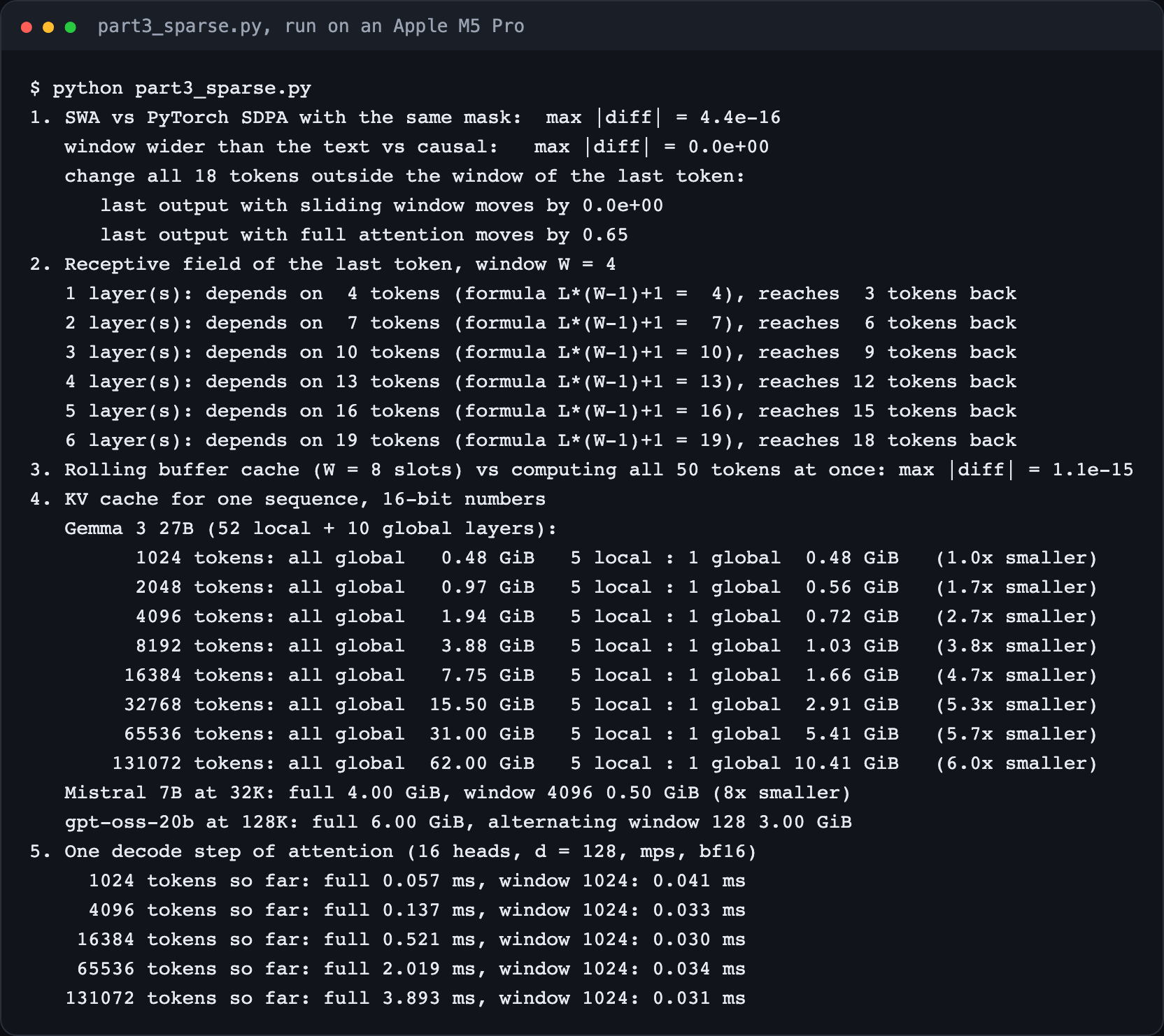
I checked three things in part3_sparse.py (24 tokens, $W = 6$, 64-bit numbers):

1. SWA vs PyTorch SDPA with the same mask:  max |diff| = 4.4e-16
   window wider than the text vs causal:   max |diff| = 0.0e+00
   change all 18 tokens outside the window of the last token:
      last output with sliding window moves by 0.0e+00
      last output with full attention moves by 0.65

1. My function agrees with PyTorch's built-in attention to $4.4 \times 10^{-16}$ (rounding noise).
2. A window wider than the text is exactly ordinary causal attention (difference 0).
3. The real test of "only the last W tokens matter": I replaced all 18 tokens outside the last token's window with random new ones. With the sliding window, the last token's output did not move at all (difference exactly 0). With full attention, it moved by 0.65.

3. "But then the model forgets everything older than W?"#

Not quite, and this is the clever part. A model has many layers stacked on top of each other. Layer 2 reads the outputs of layer 1, and each of those outputs already mixed information from its own window.

Each layer lets information travel $W - 1$ more tokens back. After $L$ layers:

The Mistral 7B paper says the same thing (counting the window with its $W+1$ convention):

Longformer (2020) wrote the same rule in its own notation, with $\ell$ layers and window $w$:

Proof. I stacked 1 to 6 sliding-window layers ($W = 4$, with the usual "add the input back" connection that real models use), and asked PyTorch which input tokens the last output depends on. It can tell exactly, by computing the gradient.

2. Receptive field of the last token, window W = 4
   1 layer(s): depends on  4 tokens (formula L*(W-1)+1 =  4), reaches  3 tokens back
   2 layer(s): depends on  7 tokens (formula L*(W-1)+1 =  7), reaches  6 tokens back
   3 layer(s): depends on 10 tokens (formula L*(W-1)+1 = 10), reaches  9 tokens back
   4 layer(s): depends on 13 tokens (formula L*(W-1)+1 = 13), reaches 12 tokens back
   5 layer(s): depends on 16 tokens (formula L*(W-1)+1 = 16), reaches 15 tokens back
   6 layer(s): depends on 19 tokens (formula L*(W-1)+1 = 19), reaches 18 tokens back

The measured reach matches the formula exactly, at every depth.

4. The rolling buffer cache: memory that never grows#

With a window, a token never needs keys and values older than $W$ steps. So the KV cache can be a fixed-size ring.

Here is the decoding loop from part3_sparse.py. It writes one token at a time into a cache of only $W$ slots:

k_cache = torch.zeros(H, W, d, dtype=torch.float64)                     # the whole cache: W slots, never more
v_cache = torch.zeros(H, W, d, dtype=torch.float64)
step_out = []
for i in range(T):
    xi = x[i:i + 1]
    qi = rope((xi @ Wq).view(1, H, d).transpose(0, 1), pos[i:i + 1])
    ki = rope((xi @ Wk).view(1, H, d).transpose(0, 1), pos[i:i + 1])
    vi = (xi @ Wv).view(1, H, d).transpose(0, 1)
    slot = i % W                                                        # position i goes to slot i mod W
    k_cache[:, slot], v_cache[:, slot] = ki[:, 0], vi[:, 0]
    n = min(i + 1, W)                                                   # how many slots are filled
    step_out.append(attend(qi, k_cache[:, :n], v_cache[:, :n], torch.ones(1, n, dtype=torch.bool)))

Notice that the slots are out of order: in the picture, slot 0 holds token 8 and slot 2 holds token 6. Does that break anything? No, for two reasons:

1. Softmax and the weighted sum do not care about order. Adding up "weight × value" over a set of tokens gives the same answer in any order.
2. Position is already baked into each key. RoPE (explained in Part 2) rotates each key by its position before it is stored, so the key remembers where it came from, whatever slot it sits in.

Proof. I compared this token-by-token ring cache with computing all 50 tokens at once using the sliding-window mask (2 heads, RoPE on):

3. Rolling buffer cache (W = 8 slots) vs computing all 50 tokens at once: max |diff| = 1.1e-15

Identical, while the cache held 8 slots instead of 50.

How much memory does it save?#

The KV cache formula from Part 2, with the number of stored tokens capped at $W$:

where $n$ is the number of tokens so far, and the other symbols are as in Part 2 (layers, key/value heads, head size, bytes per number).

For Mistral 7B (32 layers, 8 key/value heads, head size 128, window 4,096) at 32,768 tokens:

   Mistral 7B at 32K: full 4.00 GiB, window 4096 0.50 GiB (8x smaller)

And speed?#

Every writing step reads the whole cache. With full attention that read keeps growing; with a window it stays the same size. I timed one attention step (16 heads, head size 128, 16-bit numbers) on an Apple M5 Pro GPU:

At 128K tokens, the windowed step is about 125 times faster. (At 1,024 tokens both read the same amount; the small gap there is timing noise.)

5. Mixing local and global layers#

A pure sliding-window model has the weakness from the warning above: it can never look up an old token directly. The fix that most recent models use is to mix two kinds of layers:

This idea is older than chatbots. Longformer (2020) already combined the two inside one layer:

Today's models do it layer by layer:

• Gemma 2 (2024) alternates 1 local : 1 global, with a local window of 4,096 tokens.
• Gemma 3 (2025) goes further: 5 local : 1 global, and shrinks the window to 1,024.
• gpt-oss (OpenAI, 2025) alternates 1 : 1 with a tiny window of just 128 tokens.

Do the local layers hurt quality? Gemma 3 tested it:

Here is the published configuration (from Hugging Face), which is where those numbers come from:

{
  "num_hidden_layers": 62,
  "num_attention_heads": 32,
  "num_key_value_heads": 16,
  "head_dim": 128,
  "sliding_window": 1024,
  "sliding_window_pattern": 6,
  "rope_theta": 1000000.0,
  "rope_local_base_freq": 10000.0
}

sliding_window_pattern: 6 means every 6th layer is global: layers 6, 12, 18, ..., 60. That gives 10 global and 52 local layers.

The memory math#

Global layers store every token; local layers store at most $W$:

where $L_{\text{global}}$ and $L_{\text{local}}$ are the numbers of global and local layers. For Gemma 3 27B ($H_{kv} = 16$, $d_h = 128$, 2 bytes per number):

   Gemma 3 27B (52 local + 10 global layers):
         1024 tokens: all global   0.48 GiB   5 local : 1 global  0.48 GiB   (1.0x smaller)
         2048 tokens: all global   0.97 GiB   5 local : 1 global  0.56 GiB   (1.7x smaller)
         4096 tokens: all global   1.94 GiB   5 local : 1 global  0.72 GiB   (2.7x smaller)
         8192 tokens: all global   3.88 GiB   5 local : 1 global  1.03 GiB   (3.8x smaller)
        16384 tokens: all global   7.75 GiB   5 local : 1 global  1.66 GiB   (4.7x smaller)
        32768 tokens: all global  15.50 GiB   5 local : 1 global  2.91 GiB   (5.3x smaller)
        65536 tokens: all global  31.00 GiB   5 local : 1 global  5.41 GiB   (5.7x smaller)
       131072 tokens: all global  62.00 GiB   5 local : 1 global 10.41 GiB   (6.0x smaller)

Gemma 3's own measurement, for a 2B model, shows the same shape:

At the full 128K context: 62 GiB → 10.4 GiB. The savings can never pass 6.2× (62 layers ÷ 10 global layers), because the global layers still grow with the text. They become the main cost.

For gpt-oss-20b (24 layers alternating, 8 key/value heads, head size 64, window 128), at 128K tokens the cache drops from 6.00 GiB to 3.00 GiB: half the layers keep almost nothing.

The RoPE angle for pair $i$ of a head of size $d$ is

where "base" is 10,000 normally and 1,000,000 in Gemma 3's global layers. The slowest pair ($i = d/2 - 1$) has a period, in tokens, of about $2\pi \cdot \text{base}$: roughly 63,000 tokens for base 10k, roughly 6.3 million for base 1M. That is why the global layers need the larger base to tell positions apart across 128K tokens.

6. Attention sinks strike again: a real experiment#

All the models above were trained with their windows, so they learned to live with them. What happens if you take a normal model, trained with full attention, and simply force a window on it? This is what "StreamingLLM" studied, and the answer surprised people.

Remember the attention sink from Part 1: in Qwen2.5-0.5B, 68% of heads put most of their attention on the very first token, because softmax forces the weights to add up to 1 and the heads need somewhere harmless to "park" them. A sliding window cuts that first token off.

I tested this myself.

Setup (part3_qwen.py):

• Model: Qwen2.5-0.5B, trained with full attention.
• Text: four chunks of 2,048 tokens from Pride and Prejudice (public domain, from Project Gutenberg).
• I score only tokens 1,024 to 2,047, where every window really cuts something off.
• Each rule gets the same budget: each token may look at exactly 64, 256 or 1,024 tokens.
• "4 sinks + window" means: the first 4 tokens of the text, plus the most recent (budget − 4) tokens.
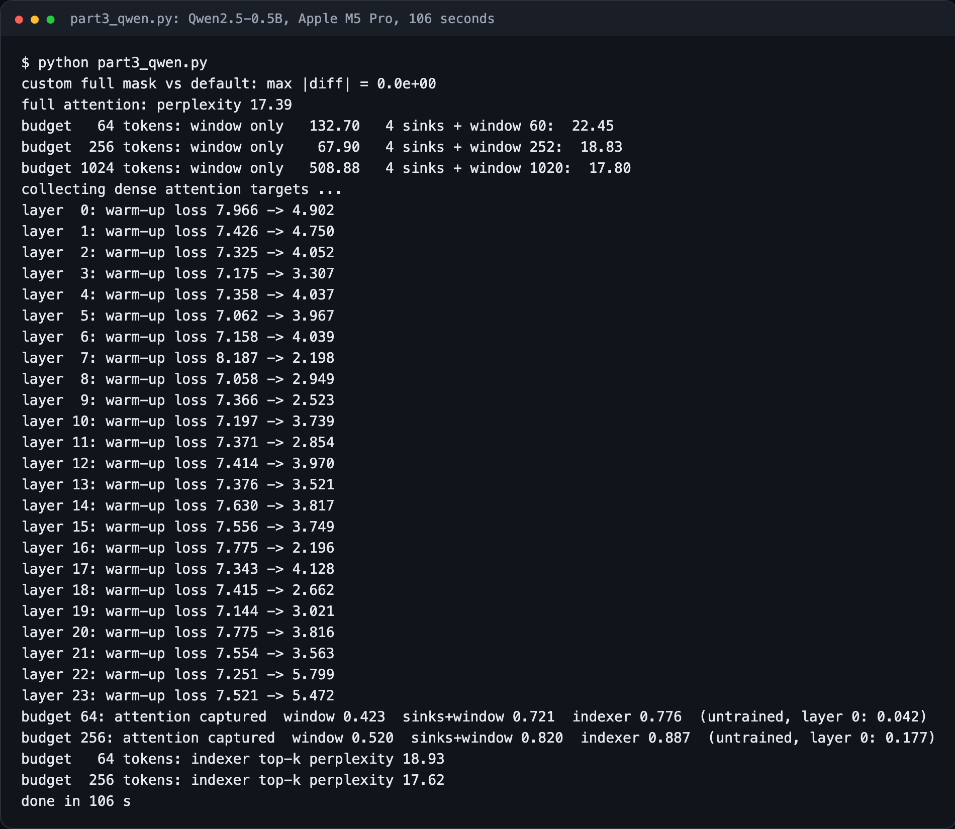
• First, a sanity check: passing my own full-attention mask gives exactly the model's normal output (max difference 0.0).

full attention: perplexity 17.39
budget   64 tokens: window only   132.70   4 sinks + window 60:  22.45
budget  256 tokens: window only    67.90   4 sinks + window 252:  18.83
budget 1024 tokens: window only   508.88   4 sinks + window 1020:  17.80

What this shows:

• A plain window destroys the model. Perplexity jumps from 17.4 to between 68 and 509.
• Keeping just 4 sink tokens fixes almost all of it. With 1,024 tokens of budget, 4 sinks plus a window give 17.80, very close to full attention's 17.39.
• A bigger window does not save you if the sink is gone. The 1,024-token window without sinks was the worst of all (508.9), even though it sees 16 times more text than the 64-token window. I did not expect this. It shows the problem is not missing information: the model is thrown off by losing its "parking spot".

With $S$ sink tokens and a window of $W$ recent tokens, the cache holds a fixed

whatever the length of the conversation: 4 + 1,020 = 1,024 tokens in my 1,024-budget test.

7. Sparse attention: let the model choose#

Windows are fixed patterns: they always keep the most recent tokens. But sometimes the important token is far away. A character's name introduced in chapter 1, a function defined at the top of a file, the original question at the start of a long chat.

Early sparse transformers (Child et al., 2019) used fixed patterns, like "the last few tokens plus every 64th token". The newer idea is to let the model pick the tokens that matter for each query. The problem: to know which tokens score highest, you seem to need the scores, which is the very thing you were trying to avoid computing.

DeepSeek's answer: compute the scores with a much smaller, much cheaper model first, then do the expensive attention only on the winners.

8. DeepSeek Sparse Attention (DSA)#

DSA arrived with DeepSeek-V3.2 (2025). It has two pieces.

Piece 1: the lightning indexer#

The index score is:

where:

• $t$ is the current (query) token and $s$ an earlier token;
• $H^I$ is the number of indexer heads (a small number);
• $q^I_{t,j}$ is the indexer query of token $t$ for indexer head $j$;
• $k^I_s$ is the indexer key of token $s$ (one key per token, shared by all indexer heads);
• $w^I_{t,j}$ is a weight that token $t$ gives to indexer head $j$ (how much to trust that head for this token);
• $\operatorname{ReLU}(x) = \max(0, x)$.

The paper explains both choices: ReLU was chosen "for throughput consideration", and the indexer "can be implemented in FP8".

Piece 2: top-k token selection#

For each query token $t$, keep only the $k$ earlier tokens with the highest index scores, and run the real attention over just those:

where:

• $I_{t,:}$ means all of token $t$'s index scores;
• $S_t$ is the set of selected positions;
• $h_t$ is the current token's hidden vector;
• $c_s$ is the cached key-value entry of token $s$ (in DeepSeek, the MLA latent from Part 2);
• $u_t$ is the attention output.

DeepSeek-V3.2 uses $k = 2{,}048$.

What it saves#

So the expensive part (the big attention with 128 heads) becomes linear in length. The cheap part (the indexer) is still quadratic, but it is so small and so fast that it costs much less.

How much less, exactly? DeepSeek-V3.2's published configuration gives the sizes: the indexer has $H^I = 64$ heads of size $d^I = 128$; the main attention has 128 heads, each scoring against a cached entry of $512 + 64 = 576$ numbers. Counting multiply-adds for the scoring step only:

where $P = L(L+1)/2$ is the number of (query, earlier token) pairs and $k = 2{,}048$. At $L = 131{,}072$ tokens:

The indexer still touches every pair, but each touch is 9 times cheaper and runs in 8-bit numbers. The main attention touches 32 times fewer pairs. (This counts only the scoring arithmetic. Real speed also depends on memory reads and GPU code; the paper's Figure 3 below shows the measured result.)

How the indexer learns: two training stages#

The indexer starts out random. How does it learn which tokens matter? It copies the model's own attention. DeepSeek trains it in two stages:

Stage 1, dense warm-up. Keep normal full attention, freeze the whole model, and train only the indexer to predict where the model's attention goes.

As an equation, with $A^{(h)}_{t,s}$ the main attention weight of head $h$ from token $t$ to token $s$:

The top sums over heads; the bottom divides by the row total so the numbers add up to 1.

The training loss compares the indexer's scores (turned into a distribution by softmax) with that target:

This stage is short: 1,000 steps, 2.1 billion tokens, learning rate $10^{-3}$.

Stage 2, sparse training. Switch on top-k selection and train the whole model to work with it: 15,000 steps, 943.7 billion tokens. The indexer keeps learning from the KL loss, but it is trained separately: the paper says "we detach the indexer input from the computational graph for separate optimization", meaning the indexer's learning signal does not flow back into the main model.

9. I trained a lightning indexer on a real model#

To see whether this really works, and not just trust the paper, I built a small DSA for Qwen2.5-0.5B and ran stage 1 (the dense warm-up) exactly as described: model frozen, indexer trained with the KL loss against the model's own head-summed, L1-normalised attention.

The indexer, one per layer, 24 in total:

• 4 indexer heads of size 32, one shared key per token, ReLU, and the weights $w$;
• RoPE on its queries and keys, so it knows positions;
• a LayerNorm on its input (more on this below);
• 148,736 parameters per layer, about 8% of the size of the attention layer it serves (1,836,160).

class LightningIndexer(torch.nn.Module):
    """I[t, s] = sum_j w[t, j] * ReLU(q[t, j] . k[s])   (DeepSeek-V3.2, eq. 1). One shared key per token."""
    def __init__(self, d_model):
        super().__init__()
        self.norm = torch.nn.LayerNorm(d_model)                        # Qwen's hidden states have a few huge values; tame them
        self.q = torch.nn.Linear(d_model, HI * DI, bias=False)
        self.k = torch.nn.Linear(d_model, DI, bias=False)
        self.w = torch.nn.Linear(d_model, HI, bias=False)

    def forward(self, h):                                              # h: (T, d_model)
        n, h = h.shape[0], self.norm(h)
        q = rope(self.q(h).view(n, HI, DI).transpose(0, 1))            # (HI, T, DI)
        k = rope(self.k(h))                                            # (T, DI)
        return torch.einsum('jt,jts->ts', self.w(h).T, F.relu(q @ k.T))   # (T, T)

The target and the loss, as in the paper (summing the 14 heads, then dividing by the total; the KL loss written as cross-entropy, which differs from KL only by a constant):

        A = output[1][0]                                               # (heads, T, T)
        captured[layer]['p'] = (A.sum(0) / A.sum(0).sum(-1, keepdim=True)).detach()   # sum over heads, L1-normalise

def kl_loss(ix, h, p):
    I = ix(h).masked_fill(~CAUSAL, float('-inf'))
    logq = torch.log_softmax(I, -1)
    return -(p * logq.masked_fill(~CAUSAL, 0)).sum(-1).mean()          # KL(p || softmax(I)) up to a constant

Training: 400 steps per layer, learning rate $10^{-3}$ (the paper's warm-up rate), on six 2,048-token chunks of The Adventures of Sherlock Holmes. Testing used a different book, Pride and Prejudice, so the indexer never saw the test text.

Result 1: does it pick the tokens the model really attends to?#

For each layer and each query token (positions 1,024 to 2,047), I measured what share of the model's real attention lands on the chosen tokens. 1.0 would mean the chosen tokens hold all of the attention.

budget 64: attention captured  window 0.423  sinks+window 0.721  indexer 0.776  (untrained, layer 0: 0.042)
budget 256: attention captured  window 0.520  sinks+window 0.820  indexer 0.887  (untrained, layer 0: 0.177)

• An untrained indexer catches almost nothing (4.2%), so the training clearly did the work.
• The trained indexer beats the strong "sinks + window" rule at both budgets. It found the sinks and the recent tokens by itself, plus some important far-away tokens.

Here is one real example: the very last token of a test chunk, in layer 13.

Result 2: does the model still work with sparse attention?#

The real test: run Qwen with every layer using top-k attention chosen by its indexer, and measure perplexity on Pride and Prejudice.

With 256 tokens per query (full attention reads 1,025 to 2,048 at these positions), the indexer version reaches 17.62, against 17.39 for full attention, without retraining the model at all. With 64 tokens it stays at 18.93, clearly better than the best fixed pattern (22.45).

10. Proof of the runs#

Both scripts, exactly as they ran (the same outputs quoted above):

The impact, and where you meet it#

Long context went from a research problem to a standard feature between 2023 and 2025, and the ideas in this part are a big reason why:

• Mistral 7B (2023) made sliding windows and the rolling cache standard in open models.
• Gemma 2 and 3, gpt-oss made local and global layers the default way to reach 128K tokens with a manageable cache.
• StreamingLLM showed how to keep a model running on a never-ending stream; keeping attention sinks is now a standard trick in serving systems.
• DeepSeek-V3.2 showed that a learned top-k selection can keep quality while cutting long-context cost sharply.

Use cases in one line each:

• Long documents (contracts, books, codebases): local and global layers keep the cache affordable at 128K tokens.
• Endless chats and live streams: a rolling window plus attention sinks keeps memory fixed for as long as the stream runs.
• Reasoning models that write tens of thousands of tokens: sparse attention (DSA) keeps each new token cheap, however long the reasoning gets.
• Retrieval inside long context ("find the clause that mentions X"): this needs global layers or a learned selector, because a pure window cannot look that far directly.

Which one to use?#

Notice that DSA still keeps every token's latent in memory (any of them might be chosen), but reads only $k$ of them per step. Sliding windows save memory too; DSA saves mainly reading and computing.

All of these still use softmax attention over some set of tokens. Part 4 goes one step further: layers that replace softmax attention with a fixed-size memory that never grows at all (linear attention, Gated DeltaNet), and the hybrid models that mix them with ordinary attention.

Summary#

• Full attention compares every token with every earlier token: $T(T+1)/2$ comparisons per head per layer, 8.6 billion at 128K tokens.
• Sliding-window attention adds one condition to the mask, $0 \le i - j < W$. I checked it against PyTorch ($4.4 \times 10^{-16}$) and showed that tokens outside the window have exactly zero effect.
• Stacked layers still see far: the reach is $L(W-1)+1$, measured exactly with gradients for 1 to 6 layers.
• A rolling buffer stores token $i$ in slot $i \bmod W$. It matched full computation to $1.1 \times 10^{-15}$, cut Mistral 7B's cache 8× at 32K, and kept a decode step flat (0.031 ms vs 3.893 ms at 128K).
• Local + global layers keep some full-attention layers for direct long-range lookups. Gemma 3 27B: 62 GiB → 10.4 GiB at 128K.
• A model trained with full attention breaks under a plain window (perplexity 17.4 → up to 509) because it loses its attention sink. Keeping 4 first tokens fixes most of it (17.80).
• DeepSeek Sparse Attention uses a tiny lightning indexer, $I_{t,s} = \sum_j w^I_{t,j}\,\operatorname{ReLU}(q^I_{t,j} \cdot k^I_s)$, to pick the top-k tokens, so the main attention costs $O(Lk)$ instead of $O(L^2)$.
• My indexer for Qwen2.5-0.5B, trained only with the warm-up KL loss, caught 77.6% of the real attention with 64 tokens and brought perplexity to 17.62 with 256 tokens (full: 17.39).
• With DeepSeek-V3.2's real sizes, DSA scores a 128K-token text with about 7× fewer multiply-adds than dense attention, and the paper's measured decode cost at 128K drops from about $2.1 to $0.25 per million tokens.

pip install torch transformers
python part3_sparse.py     # writes results/part3.json
python part3_qwen.py       # writes results/part3_qwen.json

References#

1. A. Q. Jiang et al. Mistral 7B. 2023.
2. I. Beltagy, M. E. Peters, A. Cohan. Longformer: The Long-Document Transformer. 2020.
3. R. Child, S. Gray, A. Radford, I. Sutskever. Generating Long Sequences with Sparse Transformers. 2019.
4. G. Xiao, Y. Tian, B. Chen, S. Han, M. Lewis. Efficient Streaming Language Models with Attention Sinks. ICLR 2024.
5. Gemma Team. Gemma 2: Improving Open Language Models at a Practical Size. 2024.
6. Gemma Team. Gemma 3 Technical Report. 2025.
7. DeepSeek-AI. DeepSeek-V3.2: Pushing the Frontier of Open Large Language Models. 2025.
8. Model configurations: Mistral-7B-v0.1, Gemma 3 27B, Gemma 2 9B, gpt-oss-20b, Qwen2.5-0.5B.
9. Texts: Pride and Prejudice and The Adventures of Sherlock Holmes, Project Gutenberg.