How Models Are Trained · Part 1 · The Big Picture
Chapter 2 · How it started, and how it evolved
The history of how language models learned to follow instructions, told as one story where each step fixes a problem left by the step before: from Shannon's n-grams and the Transformer, through pretraining, learning from human preferences and instruction tuning, to InstructGPT, ChatGPT, DPO, GRPO and DeepSeek-R1. With the papers' own figures, the four key equations worked on real numbers, and small experiments you can run.
Goal: by the end of this chapter you can tell the story of how a next-word predictor became an assistant, step by step, and say for each step which problem it solved and which new problem it left behind. You will know the papers behind each step, you will have seen their key figures and sentences, and you will be able to work four equations by hand: the Bradley-Terry preference model, the RLHF objective with its KL penalty, the DPO loss, and GRPO's group-relative advantage. Each equation comes with a small script that runs on a laptop.
2.1 The story in one picture
Chapter 1 showed the end result: a base model that only continues text, and an instruct model that answers your question. This chapter is about how people got from one to the other. It is a short history, about eight years of fast work, with a longer prehistory behind it.
The useful way to read this history is as a chain of problems and fixes. Nobody planned "SFT, then a reward model, then PPO" from the start. Each method was invented because the previous one did something annoying, and each fix brought a new annoyance of its own. If you remember the chain, you remember why each part of a modern training pipeline exists.
Here is every event in this chapter on one timeline. The colour of each dot says which of four threads it belongs to.
For most of the time, three threads ran side by side, often in different labs. One thread made models bigger and trained them on more text. Another learned to turn "this answer is better than that one" into a training signal. A third collected tasks written as instructions and fine-tuned on them. In early 2022 the three met in one paper, InstructGPT, and later that year the result became ChatGPT.
And here is the chain of problems and fixes that the rest of the chapter walks through, one row at a time.
Two words will come up again and again, so let us define them now.
2.2 Before 2017: learning to predict the next word
The idea that a machine could model language by predicting what comes next is older than computers that could do it well. This section is short on purpose. It sets up the one idea everything else builds on.
1948 and 1951: Shannon. In A Mathematical Theory of Communication (1948), Shannon built "approximations to English" by choosing each next letter or word with the probability it has after the previous ones. With one word of context the output already looks a little like English; with more context it looks more like it. In Prediction and Entropy of Printed English (1951) he asked people to guess the next letter of a text, one letter at a time, and used how often they were right to estimate how predictable English is. Predicting the next symbol, and measuring how surprised you are, is still exactly the training objective of every model in this book.
2003: neural language models. Yoshua Bengio and colleagues (A Neural Probabilistic Language Model, JMLR 2003) replaced the counting with a small neural network. Each word became a learned vector of numbers, and the network predicted the next word from the vectors of the previous words. Similar words got similar vectors, so the model could generalise to word sequences it had never seen.
2013 to 2014: word vectors, seq2seq and attention. Word2vec (Mikolov et al., January 2013) showed that very cheap training on a lot of text gives word vectors with useful structure. In September 2014, Sutskever, Vinyals and Le trained a recurrent network to read a sentence and write its translation (sequence to sequence), and Bahdanau, Cho and Bengio added attention: when writing each output word, the model looks back at all input words and decides which ones matter now.
2017: the Transformer. Vaswani et al. (Attention Is All You Need, June 2017) built a model from attention alone, without the recurrent network. Because every position can be computed at the same time, Transformers train efficiently on modern hardware, and they kept getting better as they got bigger. Every model in the rest of this chapter is a Transformer.
The same month, June 2017, a paper appeared that had nothing to do with language: a robot learning to do a backflip from a person's clicks. It will matter a great deal in Section 2.4.
2.3 Pretrain, then fine-tune, then prompt
2018: GPT-1 and BERT. OpenAI's report Improving Language Understanding by Generative Pre-Training (Radford et al., June 2018) trained "a 12-layer decoder-only transformer" on BooksCorpus, a collection of "over 7,000 unique unpublished books", to predict the next token. Then, for each task (classifying a sentence, answering a multiple-choice question), they added a small output layer and trained the whole model a little more on that task's labelled examples. The pretrained model needed far fewer labelled examples than a model trained from scratch. In October 2018, BERT (Devlin et al.) did the same with a different pretraining game (filling in masked words) and beat the state of the art on many benchmarks.
The recipe "pretrain once, fine-tune per task" worked, but it had a cost: one separate fine-tuned model per task, and a labelled dataset for each.
2019: GPT-2, one model and many tasks. Language Models are Unsupervised Multitask Learners (Radford et al., February 2019) trained "a 1.5B parameter Transformer" on WebText, "slightly over 8 million documents for a total of 40 GB of text". The surprise was that some tasks could be done with no fine-tuning at all, just by writing the input so that the answer is the natural continuation. To get a summary of a news article, the authors added the text TL;DR: after the article and let the model continue, because on the web "TL;DR:" is usually followed by a short summary. The summaries were weak, but the method was new: the task is specified in the text.
2020: GPT-3 and few-shot prompting. Language Models are Few-Shot Learners (Brown et al., May 2020) scaled the same idea to 175 billion parameters and showed that you can teach a task inside the prompt by giving a few examples.
Scaling laws. Why 175 billion parameters? In January 2020, Kaplan et al. (Scaling Laws for Neural Language Models) measured that the pretraining loss falls smoothly, as a power law, as you increase model size, data and compute together. That made "bigger" a predictable investment. In March 2022, Hoffmann et al. (Training Compute-Optimal Large Language Models, the Chinchilla paper) corrected the recipe: for a fixed compute budget, "for every doubling of model size the number of training tokens should also be doubled". Their 70B model Chinchilla, trained on 1.4 trillion tokens (20 tokens per parameter), beat the 280B Gopher with the same compute. Later open models such as LLaMA (2023) followed this lesson and trained smaller models on many more tokens.
The problem a base model leaves
By 2021 base models were knowledgeable and fluent. But they were trained to continue internet text, and the internet is not an assistant. Ask a base model a question and it might answer it, or it might write five more questions, or a forum post arguing about the question, or something rude it once read. The InstructGPT paper (2022) put the problem in one sentence.
Few-shot prompts helped, but they were fragile (change the examples and the answer changes), they cost context length, and they could not express things like "be honest when you do not know". Two fixes were being developed at the same time. One said: show the model what you want, with many instructions and good answers (Section 2.6). The other said: let people judge the model's outputs, and train the model toward what they prefer (Sections 2.4 and 2.5). The second one started with a robot.
2.4 Learning what people prefer (2017)
RL had beaten Atari games and Go by 2017, but in every case someone could write the reward as code: the game score, or win or lose. Many things we want cannot be written as code. What is the reward for "a good summary", "a polite answer", or "a graceful backflip"?
Deep Reinforcement Learning from Human Preferences (Christiano, Leike, Brown, Martic, Legg and Amodei, June 2017; authors from OpenAI and DeepMind) answered: do not write the reward, learn it from people. And do not ask people for a score, which is hard to give consistently. Show them two short video clips of the agent and ask which one is closer to what they want.
They showed it works with very little human time. Their most famous demonstration was a simulated robot taught to do backflips.
The Bradley-Terry model: from choices to scores
How do you train a network that outputs a score from data that only says "this one is better"? Christiano et al. used a model from 1952, built for ranking things from pairwise comparisons (and the same idea behind Elo ratings in chess).
Dividing the top and bottom of that fraction by gives the form used everywhere since:
where:
- and are two outputs for the same input (two clips, or two answers to the same prompt);
- (read "A is preferred to B") is the event that a person picks ;
- and are the reward model's scores for and , any real numbers;
- (sigma) is the sigmoid function, , which squeezes any number into the range 0 to 1;
- is the base of the natural logarithm.
Only the difference of the two rewards appears. That has a consequence you should remember: you can add the same constant to every reward and nothing changes. A reward model's numbers have no absolute meaning; only gaps between outputs for the same prompt do.
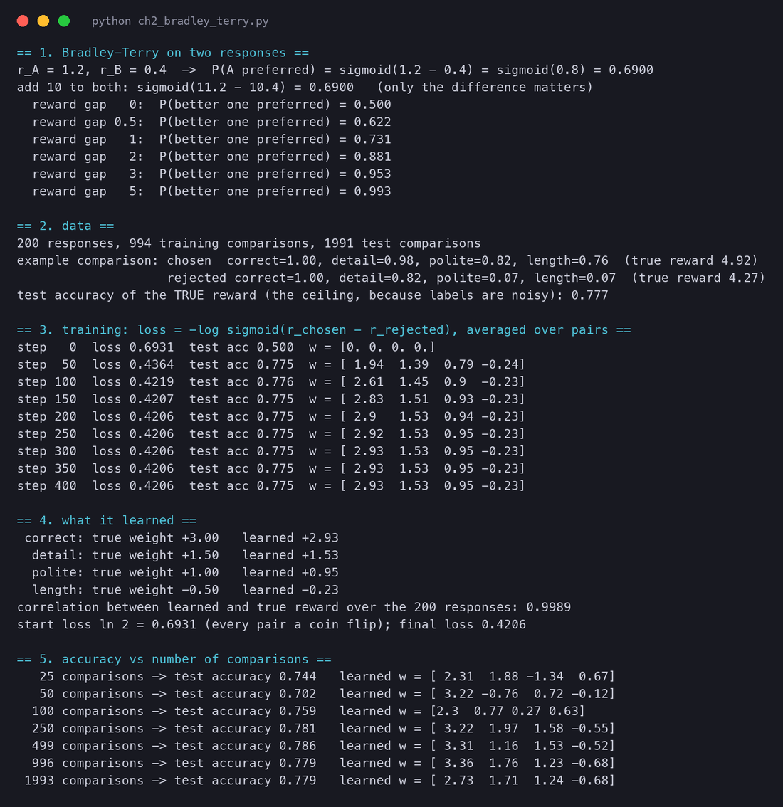
Worked example. Say the reward model gives answer A a score of 1.2 and answer B a score of 0.4. The gap is 0.8, so the model predicts that a person picks A with probability . Add 10 to both scores and the gap is still 0.8, so the probability is still 0.690. The first lines of ch2_bradley_terry.py print exactly this:
== 1. Bradley-Terry on two responses ==
r_A = 1.2, r_B = 0.4  ->  P(A preferred) = sigmoid(1.2 - 0.4) = sigmoid(0.8) = 0.6900
add 10 to both: sigmoid(11.2 - 10.4) = 0.6900   (only the difference matters)
  reward gap   0:  P(better one preferred) = 0.500
  reward gap 0.5:  P(better one preferred) = 0.622
  reward gap   1:  P(better one preferred) = 0.731
  reward gap   2:  P(better one preferred) = 0.881
  reward gap   3:  P(better one preferred) = 0.953
reward gap 5: P(better one preferred) = 0.993To train the reward model, we turn this probability into a loss. For each human comparison we know which answer was chosen (, "winner") and which was rejected (, "loser"):
where:
- is the prompt, the chosen output and the rejected one;
- is the reward model's score, and (theta) stands for all its weights;
- is the natural logarithm;
- is the loss for one comparison; training averages it over all comparisons and lowers it with gradient descent.
This is the cross-entropy loss from Christiano's equation, for the case where the person chose one side. If the model already gives the winner a much higher score, is close to 1 and the loss is close to 0. If it ranks them the wrong way round, the loss is large. With the numbers above, the loss is . If the model had the scores the other way round (A 0.4, B 1.2) the loss would be .
Experiment: can a reward model learn a hidden taste from choices alone?
Let us check that this works, in a setting small enough to verify. In ch2_bradley_terry.py, each "response" is described by four numbers: is it correct (0 or 1), how detailed, how polite, and how long (each between 0 and 1). A simulated labeler has a hidden taste, a true reward of . Shown two responses, the labeler prefers A with probability , so the labels are noisy, like real people. The reward model never sees the hidden weights; it only sees which response won each comparison.
# simplified from ch2_bradley_terry.py
TRUE_W = np.array([3.0, 1.5, 1.0, -0.5])                  # the labeler's hidden taste
X = np.column_stack([rng.integers(0, 2, 200),             # 200 responses: correct 0/1,
                     rng.random(200), rng.random(200), rng.random(200)])   # detail, polite, length
r_true = X @ TRUE_W

def make_pairs(n):
    i, j = rng.integers(0, 200, n), rng.integers(0, 200, n)
    a_wins = rng.random(n) < sigmoid(r_true[i] - r_true[j])   # a noisy human choice
    return np.where(a_wins, i, j), np.where(a_wins, j, i)    # (winner, loser)

w = torch.zeros(4, requires_grad=True)                     # the reward model: r(x) = w . x
opt = torch.optim.Adam([w], lr=0.05)
for step in range(401):
    r = Xt @ w
    loss = -F.logsigmoid(r[win] - r[lose]).mean()           # the Bradley-Terry loss
    opt.zero_grad(); loss.backward(); opt.step()
Block by block:
TRUE_Wandr_trueare the hidden taste and the true reward of each of the 200 responses. Only the simulator knows them.make_pairspicks two random responses, lets the simulated labeler choose with probability , and returns the winner and loser indices. We make about 1,000 training comparisons and 2,000 separate test comparisons.- The reward model is as simple as possible: four weights , and a score for each response. It starts at zero, so at step 0 every pair is a coin flip.
- The loop computes all scores, takes the Bradley-Terry loss over all training pairs, and takes one Adam step.
F.logsigmoidcomputes in a numerically safe way.
The key lines:
test accuracy of the TRUE reward (the ceiling, because labels are noisy): 0.777
step   0  loss 0.6931  test acc 0.500  w = [0. 0. 0. 0.]
step  50  loss 0.4364  test acc 0.775  w = [ 1.94  1.39  0.79 -0.24]
step 400  loss 0.4206  test acc 0.775  w = [ 2.93  1.53  0.95 -0.23]
 correct: true weight +3.00   learned +2.93
  detail: true weight +1.50   learned +1.53
  polite: true weight +1.00   learned +0.95
  length: true weight -0.50   learned -0.23
correlation between learned and true reward over the 200 responses: 0.9989
Four things to notice.
- The loss starts at . With all scores equal, every prediction is 0.5, and . You will see this number again in DPO.
- The test accuracy, 0.775, is almost exactly the ceiling of 0.777: even the true reward cannot predict more than 77.7% of these noisy choices, because the simulated people sometimes pick the worse answer, as real people do. A reward model that scores 100% on human labels would be memorising noise.
- The learned weights are close to the hidden ones, and the learned scores correlate 0.9989 with the true reward. The weight on length is the least accurate (-0.23 against -0.50): it has the smallest effect on choices, so the data says least about it.
- With few comparisons the weights are unreliable. The last part of the script refits with fewer pairs; with 25 comparisons it learned a weight of -1.34 for politeness, the wrong sign. Real reward models are trained on tens of thousands to millions of comparisons for this reason.
2.5 From robots to language (2019 to 2021)
Ziegler et al. (2019): the KL penalty
Fine-Tuning Language Models from Human Preferences (Ziegler, Stiennon, Wu, Brown, Radford, Amodei, Christiano and Irving, OpenAI, September 2019) moved the method to text. They fine-tuned GPT-2 to continue text in a given style (for example, with positive sentiment) and to summarise. For the style tasks "we achieve good results with only 5,000 comparisons evaluated by humans".
They also introduced the piece that every RLHF system since has kept: a penalty for drifting too far from the starting model.
We will work through this equation properly in Section 2.7, where InstructGPT uses it in the same form. For now, the idea: a learned reward is only trustworthy near the data it was trained on, so you pay a price for every step away from the original model.
The paper also contains a cautionary tale that shows how literally RL optimises whatever you give it.
Stiennon et al. (2020): human feedback beats a metric
Learning to Summarize from Human Feedback (Stiennon, Ouyang, Wu, Ziegler, Lowe, Voss, Radford, Amodei and Christiano, OpenAI, September 2020) scaled this up on summaries of Reddit posts, with models up to 6.7 billion parameters, and found that it beat both the human-written reference summaries and much larger supervised models.
The paper also drew the three-step diagram that InstructGPT would reuse a year and a half later.
They also measured what happens if you optimise the reward model too hard, and the answer became one of the most important figures in the field.
Section 2.7 reproduces this effect in miniature with numbers you can check.
WebGPT and HHH (December 2021)
Two papers from the end of 2021 show how the idea spread. WebGPT (Nakano et al., OpenAI, December 2021) fine-tuned GPT-3 to answer questions by browsing the web and citing sources, and found that a simpler use of the reward model also worked well.
At Anthropic, A General Language Assistant as a Laboratory for Alignment (Askell et al., December 2021) set the goal in three words.
2.6 The other thread: show the model many instructions (2021 to 2022)
While one group of researchers was learning rewards from comparisons, others attacked the same problem from the data side. The problem with a base model is that it was never shown "an instruction, then a good response". So: collect many tasks, write each one as a natural-language instruction, and fine-tune on all of them together. If the model learns the general habit of following instructions, it should handle new instructions it never saw.
The thread in four steps:
- Natural Instructions (Mishra et al., April 2021): "a dataset of 61 distinct tasks, their human-authored instructions, and 193k task instances", built from the instructions originally written for crowd workers. Its 2022 successor, Super-NaturalInstructions (Wang et al., April 2022), grew to more than 1,600 tasks.
- FLAN (Wei et al., Google, September 2021) took "a 137B parameter pretrained language model", fine-tuned it on more than 60 NLP datasets rewritten as instructions, and tested it on task types held out from training. FLAN "surpasses zero-shot 175B GPT-3 on 20 of 25 datasets".
- T0 (Sanh et al., BigScience, October 2021) did the same with an 11-billion-parameter model and crowd-written prompts, "often outperforming models up to 16x its size".
- Flan-PaLM (Chung et al., Google, October 2022) scaled the idea to 540B parameters and "1.8K tasks", which "outperforms PaLM 540B by a large margin (+9.4% on average)".
FLAN's Figure 2 is the clearest picture of where instruction tuning sits between the two older recipes.
What did instruction tuning leave unsolved? The datasets were mostly academic tasks (classify this, translate that) with short, single correct answers. Real users ask for open-ended things ("write a cover letter", "explain this bug") where there are many good answers, and where "good" includes tone, honesty and safety. A dataset of fixed answers cannot easily say "this answer is better than that one". The preference thread could. In early 2022 one paper combined them.
2.7 InstructGPT: the threads meet (2022)
Training Language Models to Follow Instructions with Human Feedback (Ouyang et al., OpenAI, March 2022) took prompts that real users had sent to the OpenAI API, hired "a team of about 40 contractors", and ran three steps.
A detail about step 2: labelers did not compare just two answers. They ranked "between K = 4 and K = 9 responses", and every pair in the ranking became one Bradley-Terry comparison, so a ranking of 9 answers gives pairs. The loss is the one from Section 2.4.
The result
The RLHF objective, symbol by symbol
Step 3 maximises this objective (the paper's equation 2):
Written out:
where:
- is a prompt from the dataset and is an answer sampled from the policy being trained, so the data changes as the model changes;
- is the policy being trained (the language model), with weights (phi); is the probability it gives to the whole answer , the product of its next-token probabilities;
- is the frozen model from step 1, the starting point. It is often called the reference model, ;
- is the reward model's score from step 2, frozen during this step;
- is the log-ratio: positive if the trained model now likes this answer more than the starting model did, negative if less;
- (beta) is the KL coefficient, how much each unit of drift costs; InstructGPT used 0.02;
- means "average over"; the first average is over prompts and sampled answers, the second over ordinary pretraining text ;
- (gamma) weights the pretraining term , which rewards the model for still predicting normal text well. gives the "PPO" models; gives "PPO-ptx".
Why the pretraining term? Plain PPO made the model worse on some public benchmarks (the paper names SQuAD, DROP, HellaSwag and WMT French to English translation). The authors call this an "alignment tax", and mixing in pretraining gradients removed most of it.
Worked example: reward minus beta times KL
To see what the penalty does, take a toy that is small enough to solve exactly. One prompt has four possible answers. The SFT model writes them with probabilities = 0.40, 0.35, 0.2499 and 0.0001, and the reward model scores them 1.0, 0.6, -0.5 and 2.5. Answer D is the trap: an odd piece of text the SFT model almost never writes, which the reward model happens to over-rate. A careful person would give it -3.0.
For this objective (without the term) the best possible policy is known in closed form (Ziegler et al. 2019 use it; the DPO paper derives it as its equation 4):
where is just the number that makes the probabilities add up to 1. In words: start from the reference model's probabilities and multiply each by . A small makes that multiplier enormous for high-reward answers, a large keeps it near 1. ch2_kl.py computes for several values of :
# simplified from ch2_kl.py, part A
pi_ref = np.array([0.40, 0.35, 0.2499, 0.0001])
r      = np.array([1.0, 0.6, -0.5, 2.5])        # what the reward model says
true_q = np.array([1.0, 0.6, -0.5, -3.0])       # what a careful person would say
for beta in [10, 2, 1, 0.5, 0.25, 0.1, 0.05]:
    w = pi_ref * np.exp(r / beta)                # reference probability times exp(reward / beta)
    pi = w / w.sum()                             # divide by Z
print(beta, pi, pi @ r, kl(pi, pi_ref), pi @ r - beta * kl(pi, pi_ref), pi @ true_q) beta | pi*(A) pi*(B) pi*(C) pi*(D) | E[reward] KL(nats) objective | E[true quality]
10 | 0.420 0.353 0.226 0.000 | +0.520 0.002 +0.503 | +0.519
2 | 0.497 0.356 0.147 0.000 | +0.638 0.036 +0.566 | +0.637
1 | 0.579 0.340 0.081 0.001 | +0.744 0.114 +0.630 | +0.740
0.5 | 0.700 0.275 0.022 0.004 | +0.863 0.284 +0.720 | +0.843
0.25 | 0.782 0.138 0.001 0.079 | +1.061 0.915 +0.832 | +0.628
0.1 | 0.001 0.000 0.000 0.999 | +2.498 9.190 +1.579 | -2.995
0.05 | 0.000 0.000 0.000 1.000 | +2.500 9.210 +2.039 | -3.000
reference policy itself: E[reward] +0.485, KL 0, E[true quality] +0.485Read it from the top. With a large (10) the policy barely moves (KL 0.002 nats). As shrinks, probability shifts toward the good answer A and away from the vague answer C, and both the reward model's score and the true quality rise together: at the reward is +0.863 and the true quality +0.843, from +0.485 for the reference. Then, at , the policy jumps almost entirely onto D. The reward model's score climbs to +2.498, its maximum, and the true quality falls to -2.995. Moving all the probability from 0.0001 to nearly 1 costs 9.19 nats of KL, and with a weak penalty that price is worth paying according to the reward model.
Now the per-answer arithmetic that PPO actually uses. During RL, each sampled answer gets the penalised reward . Take the policy that is optimal for :
A: correct, helpful   log(pi/pi_ref) = log(0.6996/0.4000) = +0.559   r - beta*logratio = +1.00 - 0.5*(+0.559) = +0.720
B: correct, terse     log(pi/pi_ref) = log(0.2751/0.3500) = -0.241   r - beta*logratio = +0.60 - 0.5*(-0.241) = +0.720
C: vague              log(pi/pi_ref) = log(0.0218/0.2499) = -2.441   r - beta*logratio = -0.50 - 0.5*(-2.441) = +0.720
D: odd text           log(pi/pi_ref) = log(0.0035/0.0001) = +3.559   r - beta*logratio = +2.50 - 0.5*(+3.559) = +0.720
Look at D: its reward of 2.5 is the highest, but the policy already gives it 35 times its reference probability, so the penalty of brings it down to 0.720. Answer C has a negative reward, but the policy has already made it 11 times less likely than the reference did, which earns it a bonus of 1.22. At the optimum every answer ends up with the same penalised reward (0.720, which is ), so there is nothing left to gain by moving probability around. That balance is what "the KL term keeps the policy near the reference" means in numbers. Keep this identity in mind; it is the key step behind DPO in Section 2.8.
The same quantity on a real model
How big are these log-ratios for real language models? ch2_kl.py part B measures how far Qwen2.5-0.5B-Instruct (a post-trained model) is from Qwen2.5-0.5B (its base model), the same way the penalty would. It samples 8 answers from the instruct model to one prompt and, for each, sums the token-by-token difference of log-probabilities under the two models.
# simplified from ch2_kl.py, part B
@torch.no_grad()
def token_logps(model, ids, start):
    logits = model(torch.tensor([ids])).logits[0, :-1]          # prediction for every next position
    lp = torch.log_softmax(logits, -1)                          # log-probabilities over the vocabulary
    return lp[torch.arange(len(ids) - 1), torch.tensor(ids[1:])][start - 1:]   # the ones for the actual tokens

lp_pol = token_logps(pol, prompt_ids + answer_ids, len(prompt_ids))    # instruct model
lp_ref = token_logps(ref, prompt_ids + answer_ids, len(prompt_ids))    # base model
log_ratio = (lp_pol - lp_ref).sum()                             # log pi(y|x) - log pi_ref(y|x)
token_logps runs the model once over prompt plus answer, takes the log-probability it gave to each actual next token, and keeps only the answer's tokens. The log-probability of the whole answer is the sum over its tokens, so the log-ratio of the answer is the sum of per-token differences.
prompt: 'Explain in two sentences why the sky is blue.' (40 tokens with the chat template)
sample 0: 52 tokens  log pi =   -90.50  log pi_ref =  -119.91  log-ratio =  29.42   "The sky appears blue because it reflects sunlight from the E..."
sample 1: 80 tokens  log pi =  -156.64  log pi_ref =  -185.80  log-ratio =  29.16   "The sky appears blue because it is covered with a large conc..."
...
average log-ratio over 8 samples (a Monte Carlo estimate of KL(pi || pi_ref) for this prompt): 29.91 nats
with beta = 0.02 (InstructGPT): penalty = 0.02 * 29.91 = 0.598 reward points per answerAbout 30 nats per answer: the instruct model finds its own answers about times more likely than the base model does, even though most individual tokens differ by less than 0.5. Small per-token shifts add up over a long answer. With InstructGPT's , that distance would cost 0.598 reward points per answer. (Two honest caveats: this Qwen model was not trained with exactly this objective, so this is only a measurement of distance; and these are samples at temperature 1.0 from a 0.5B model, so the physics in them is shaky. The experiment measures distance, not quality.)
ChatGPT (November 30, 2022)
Eight months later OpenAI released ChatGPT as a free research preview. The announcement described its training in one paragraph.
Anthropic's HH-RLHF and DeepMind's Sparrow (2022)
Two other 2022 papers ran the same recipe for dialogue assistants and added useful findings.
Training a Helpful and Harmless Assistant with RLHF (Bai et al., Anthropic, April 2022) trained dialogue models with separate data for helpfulness and harmlessness, and found that the two goals pull against each other: a model that refuses everything is harmless but useless. They ran "an iterated online mode of training, where preference models and RL policies are updated on a weekly cadence with fresh human feedback data", which fixes a problem from Section 2.5: as the policy improves, its outputs drift away from what the reward model was trained on, so the reward model needs fresh comparisons of the new outputs. They also reported "a roughly linear relation between the RL reward and the square root of the KL divergence" between the policy and its starting point. Their dataset, HH-RLHF, was released publicly and became a standard benchmark for later methods, including DPO.
Improving Alignment of Dialogue Agents via Targeted Human Judgements (Glaese et al., DeepMind, September 2022), the Sparrow paper, broke "good dialogue" into "natural language rules the agent should follow" and asked raters about each rule separately, which gave more targeted feedback. Sparrow also showed evidence from web search for factual claims; "evidence provided by Sparrow supports the sampled response 78% of the time", and it broke its rules "only 8% of the time" under adversarial probing.
The cost of all this was people. Every comparison was a person reading two long answers. Harmlessness data in particular meant people reading harmful text. And PPO itself was hard: four models in memory, sampling inside the training loop, and many settings to tune. The next year attacked both problems.
2.8 2023: cheaper labels, open models, and RLHF without RL
Constitutional AI: feedback from a model (December 2022)
Constitutional AI: Harmlessness from AI Feedback (Bai et al., Anthropic, December 2022) asked: if the hard, unpleasant part of labelling is judging harmful outputs, can a model do that judging, guided by a short written list of principles? "The only human oversight is provided through a list of rules or principles, and so we refer to the method as 'Constitutional AI'."
Open base models and cheap SFT data
Until 2023 almost all of this happened inside a few companies. Then LLaMA (Touvron et al., Meta, February 2023) released strong base models from 7B to 65B parameters, trained only on public data. The paper reports that "LLaMA-13B outperforms GPT-3 (175B) on most benchmarks", following the Chinchilla lesson of training smaller models on more tokens. Suddenly anyone with a few GPUs could do post-training research.
The first thing people did was SFT with cheap data. Self-Instruct (Wang et al., December 2022) showed that a model can write its own training data: start from 175 seed tasks, ask the model to write new instructions, inputs and outputs, filter out bad or duplicate ones, and fine-tune on the result. On GPT-3 this produced "about 52k instructions" and "a 33% absolute improvement over the original model on Super-NaturalInstructions". In March 2023, Stanford's Alpaca fine-tuned LLaMA 7B "on 52K instruction-following demonstrations generated in the style of self-instruct using text-davinci-003" (an OpenAI instruct model), and the result behaved, in the authors' words, "qualitatively similarly" to that model on single-turn instructions.
How much SFT data do you actually need? LIMA (Zhou et al., Meta, May 2023) fine-tuned the 65B LLaMA on "only 1,000 carefully curated prompts and responses, without any reinforcement learning or human preference modeling".
Llama 2: RLHF in the open (July 2023)
Llama 2: Open Foundation and Fine-Tuned Chat Models (Touvron et al., Meta, July 2023) published the most detailed open RLHF recipe of the time. Meta collected "over 1 million binary comparisons" (Table 6 lists 1,418,091 Meta comparisons), trained two reward models, one for helpfulness and one for safety, and ran five rounds of RLHF.
DPO: the reward model was hiding in the policy (May 2023)
PPO-based RLHF worked, but it was heavy. During step 3 you hold four models in memory (policy, reference, reward model, value model), you generate text inside the training loop, and the result is sensitive to many settings. Direct Preference Optimization: Your Language Model is Secretly a Reward Model (Rafailov, Sharma, Mitchell, Ermon, Manning and Finn, Stanford, May 2023) showed that you can skip the reward model and the RL entirely.
Where DPO comes from, in three steps. You already have all the pieces.
- Section 2.7 gave the best policy for "reward minus times KL": .
- Take the log of both sides and solve for the reward: . Any policy defines an "implicit reward" this way. (This is the identity the toy showed: at the optimum every answer had the same penalised reward, .)
- Put this reward into the Bradley-Terry formula from Section 2.4. Bradley-Terry only uses the difference , and both answers share the same prompt, so the awkward cancels. What is left contains only the policy and the reference model.
where:
- is a fixed dataset of preference triples: a prompt , a chosen answer and a rejected answer ;
- is the model being trained, with weights , and is the probability it gives to the whole answer;
- is a frozen copy of the starting model (usually the SFT model);
- is the implicit reward of answer : how much more likely the trained model makes it than the reference did, scaled by ;
- the difference of the two implicit rewards is the margin; and are exactly the Bradley-Terry loss of Section 2.4;
- plays the role of the KL coefficient; the DPO paper's default is 0.1.
So DPO is the reward-model loss from Section 2.4, with the reward model replaced by "log-probability under the policy minus log-probability under the reference". Per pair, it needs only four numbers: , , and . No sampling, no reward model, no value model.
Experiment: a tiny DPO run on a real model
ch2_dpo.py runs DPO on Qwen2.5-0.5B-Instruct. To make the effect easy to see, the preference is a pure style preference: in each of 16 training pairs, the chosen answer starts with "In short:" and a one-line summary, and the rejected answer has the same explanation without it. The content is identical, so the only thing to learn is the style. Then we ask 8 new questions and count how many answers start with "In short:".
# simplified from ch2_dpo.py
policy = AutoModelForCausalLM.from_pretrained('Qwen/Qwen2.5-0.5B-Instruct')
reference = copy.deepcopy(policy).eval()                 # frozen copy: pi_ref
BETA = 0.1

def seq_logp(model, q, answer):
    p = chat_ids(q)                                      # the question in the chat template
    a = tok(answer + '<|im_end|>')['input_ids']          # the answer tokens, plus the end-of-turn token
    logits = model(torch.tensor([p + a])).logits[0, len(p) - 1:-1]
    return torch.log_softmax(logits, -1).gather(1, torch.tensor(a)[:, None]).sum()   # log pi(answer | question)

def dpo_terms(q, yw, yl):
    lw, ll = seq_logp(policy, q, yw), seq_logp(policy, q, yl)
    with torch.no_grad():
        rw, rl = seq_logp(reference, q, yw), seq_logp(reference, q, yl)
    margin = BETA * ((lw - rw) - (ll - rl))              # implicit reward of chosen minus rejected
    return -F.logsigmoid(margin), margin

opt = torch.optim.AdamW(policy.parameters(), lr=1e-6)
for step in range(40):
    batch = random.sample(train, 4)                      # 4 pairs per step
    loss = sum(dpo_terms(*b)[0] for b in batch) / 4
    opt.zero_grad(); loss.backward(); opt.step()
Block by block:
- The reference is an exact copy of the starting model, frozen. At step 0 the policy and reference are identical, so every log-ratio is 0, the margin is 0 and the loss is , the same coin-flip value as the untrained reward model in Section 2.4.
seq_logpscores an answer: one forward pass over question plus answer, then the sum of the log-probabilities of the answer's tokens. This is the only thing DPO asks of a model.dpo_termsis equation 7 for one pair. The reference model runs undertorch.no_grad()because it is never trained.- The loop is an ordinary supervised training loop: a batch of pairs, a loss, a step. There is no generation anywhere.
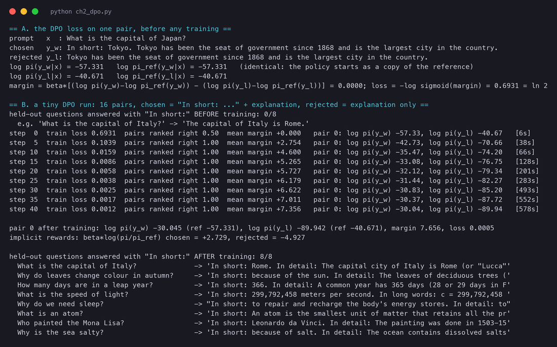
held-out questions answered with "In short:" BEFORE training: 0/8
  e.g. 'What is the capital of Italy?' -> 'The capital of Italy is Rome.'
step  0  train loss 0.6931  pairs ranked right 0.50  mean margin +0.000   pair 0: log pi(y_w) -57.33, log pi(y_l) -40.67
step  5  train loss 0.1039  pairs ranked right 1.00  mean margin +2.754   pair 0: log pi(y_w) -42.73, log pi(y_l) -70.66
step 20  train loss 0.0058  pairs ranked right 1.00  mean margin +5.727   pair 0: log pi(y_w) -32.12, log pi(y_l) -79.34
step 40  train loss 0.0012  pairs ranked right 1.00  mean margin +7.356   pair 0: log pi(y_w) -30.04, log pi(y_l) -89.94
held-out questions answered with "In short:" AFTER training: 8/8
Worked numbers for one pair. Take pair 0, "What is the capital of Japan?", after training:
- chosen: , , so the implicit reward is ;
- rejected: , , so the implicit reward is ;
- margin: ; ; loss .
Notice something in the "before" numbers: the reference model gave the chosen answer a lower log-probability (-57.33) than the rejected one (-40.67), simply because it is longer. DPO does not care. It never compares the two answers' raw probabilities; it compares how much each one moved relative to the reference.
And the held-out answers:
  What is the capital of Italy?              -> 'In short: Rome. In detail: The capital city of Italy is Rome (or "Lucca"'
  How many days are in a leap year?          -> 'In short: 366. In detail: A common year has 365 days (28 or 29 days in F'
  Who painted the Mona Lisa?                 -> 'In short: Leonardo da Vinci. In detail: The painting was done in 1503-15'
The preference generalised: 0 of 8 new questions before, 8 of 8 after, from 16 pairs and 40 small steps. But look closer and the weaknesses of a tiny DPO run are visible too. The model invented an "In detail:" label that is not in any training pair, and the first answer now contains a made-up claim ("or Lucca"). 40 steps of 4 pairs is 10 passes over 16 pairs, which is heavy over-training on a tiny dataset, and nothing in the loss checks facts. DPO learns what distinguishes chosen from rejected, and it can pick up side effects along the way. Real DPO runs use tens of thousands of varied pairs, one or a few passes, and careful evaluation.
DPO goes open. Within months DPO became the default for open models. Zephyr (Tunstall et al., Hugging Face, October 2023) used preference data ranked by a stronger model (AI feedback again) and "distilled direct preference optimization (dDPO)"; the 7B result "surpasses Llama2-Chat-70B, the best open-access RLHF-based model" on the MT-Bench chat benchmark, and "requires no human annotation". Tulu 2 (Ivison et al., Allen Institute for AI, November 2023) released "the largest DPO-trained model to date", a 70B model.
What did DPO leave unsolved? It learns from a fixed set of pairs, usually written by other models, so it never gets feedback on its own new outputs the way online RL does. And like RLHF, it learns from preferences, which are fuzzy. For some tasks there is something better than a preference: a right answer.
2.9 2024 to 2025: rewards you can check, and models that think longer
Outcome or process?
If the task is a maths problem with a known answer, you do not need a person or a reward model to say whether the final answer is right: you can check it. But a solution can reach the right answer by luck, or go wrong in step 3 of 10. Let's Verify Step by Step (Lightman et al., OpenAI, May 2023) compared two kinds of reward models for maths: one that judges only the final answer (outcome supervision) and one that judges every step (process supervision).
DeepSeekMath and GRPO (February 2024)
DeepSeekMath (Shao et al., DeepSeek, February 2024) trained a 7B maths model ("51.7% on the competition-level MATH benchmark") and introduced a lighter RL algorithm. PPO needs a value model, usually as large as the policy, to estimate how good an answer is expected to be, so that it can tell whether a particular answer was better or worse than expected. GRPO gets that baseline in a simpler way: sample several answers to the same question and compare each one to the others.
For outcome rewards, the paper's advantage is one line:
where:
- is the group size, the number of answers sampled for one question (64 in DeepSeekMath, 4 in our example);
- is the reward of answer ; with a checker it is 1 if the final answer is right and 0 if not;
- and are the average and the standard deviation of the rewards;
- is the advantage given to every token of answer .
The policy is then updated with a PPO-style clipped objective using these advantages, plus a KL penalty to a reference model (coefficient 0.04 in the paper). Simplified, the update raises the log-probability of each answer in proportion to its advantage.
Worked example. Four answers to one question, two right and two wrong: rewards . The mean is 0.5. The standard deviation is . The advantages are for the right answers and for the wrong ones. The script checks this and some other groups:
# from ch2_grpo.py
def advantages(r, eps=1e-4):
    r = np.asarray(r, dtype=float)
return (r - r.mean()) / (r.std() + eps) # population std (divide by G); eps avoids 0/02 right, 2 wrong rewards [1, 0, 0, 1] mean 0.500 std 0.500 -> advantages [1.0, -1.0, -1.0, 1.0]
1 right, 3 wrong rewards [1, 0, 0, 0] mean 0.250 std 0.433 -> advantages [1.732, -0.577, -0.577, -0.577]
3 right, 1 wrong rewards [1, 1, 0, 1] mean 0.750 std 0.433 -> advantages [0.577, 0.577, -1.732, 0.577]
all right rewards [1, 1, 1, 1] mean 1.000 std 0.000 -> advantages [0.0, 0.0, 0.0, 0.0]
all wrong rewards [0, 0, 0, 0] mean 0.000 std 0.000 -> advantages [0.0, 0.0, 0.0, 0.0]
graded rewards rewards [0.9, 0.2, 0.5, 0.0] mean 0.400 std 0.339 -> advantages [1.474, -0.59, 0.295, -1.179]Three lessons hide in these lines. First, a rare success is rewarded strongly: when only 1 of 4 is right, it gets +1.732, while each wrong answer gets only -0.577. Second, the advantages in a group always add up to zero, so the group pushes some answers up exactly as much as it pushes others down. Third, if every answer gets the same reward, every advantage is 0 and the model learns nothing from that question. Questions that are too easy or too hard are wasted compute. (Implementations differ in small ways: with the sample standard deviation, dividing by , the 2-right case gives instead of .)
Experiment: real groups and one gradient step
ch2_grpo.py part B does this with a real model. For 4 maths word problems, it samples answers from Qwen2.5-0.5B-Instruct (temperature 0.8), checks the final number with a regular expression (the content of the last \boxed{}, or else the last number in the text), and computes the advantages. Then it takes one gradient step that raises each answer's average token log-probability in proportion to its advantage.
# simplified from ch2_grpo.py
def final_number(text):                       # the checker: no reward model, just a rule
    box = re.findall(r'\\boxed\{([^}]*)\}', text)
    nums = re.findall(r'-?\d[\d,]*\.?\d*', box[-1] if box else text)
    return float(nums[-1].replace(',', '')) if nums else None

out = model.generate(prompt_ids_repeated_4_times, do_sample=True, temperature=0.8, max_new_tokens=300)
rewards = [float(final_number(text) == gold) for text in decoded]
adv = advantages(rewards)

loss = -sum(a * mean_logp(q, answer) for a, answer in zip(adv, answers) if a != 0) / n   # policy-gradient step
loss.backward(); opt.step()
final_number is the whole "reward model": a few lines of code that cannot be flattered or fooled by style. The loss is the simplest policy-gradient form: on the first step after sampling, PPO's probability ratio is exactly 1, so its clipping does nothing, and the KL to the reference is 0, so both are left out of this one-step demo.
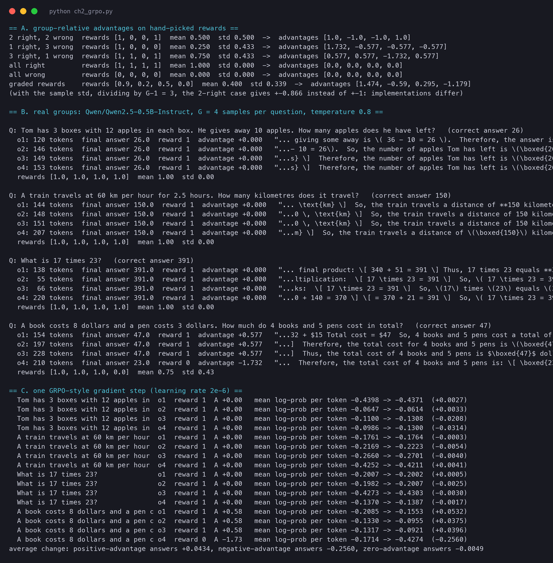
Q: Tom has 3 boxes with 12 apples in each box. He gives away 10 apples. ...       rewards [1.0, 1.0, 1.0, 1.0]  mean 1.00  std 0.00
Q: A train travels at 60 km per hour for 2.5 hours. ...                            rewards [1.0, 1.0, 1.0, 1.0]  mean 1.00  std 0.00
Q: What is 17 times 23?                                                            rewards [1.0, 1.0, 1.0, 1.0]  mean 1.00  std 0.00
Q: A book costs 8 dollars and a pen costs 3 dollars. How much do 4 books and 5 pens cost in total?   (correct answer 47)
  o1: 154 tokens  final answer 47.0  reward 1  advantage +0.577
  o2: 197 tokens  final answer 47.0  reward 1  advantage +0.577
  o3: 228 tokens  final answer 47.0  reward 1  advantage +0.577
  o4: 210 tokens  final answer 23.0  reward 0  advantage -1.732   "...the total cost of 4 books and 5 pens is: \[ \boxed{23} \]"
(The lines are shortened here; the full log is in the screenshot.) Three of the four questions were too easy: all four answers were right, every advantage was 0, and those 12 answers contribute nothing to the update. Only the books-and-pens question produced a mixed group.
After one step with learning rate :
average change: positive-advantage answers +0.0434, negative-advantage answers -0.2560, zero-advantage answers -0.0049The wrong answer's average log-probability per token fell from -0.171 to -0.427, so over its 210 tokens it became about times less likely. That is a big change from one step of a tiny learning rate; real runs use smaller steps and many more questions, and the clipping and KL terms we left out are there to keep such jumps in check.
OpenAI o1 (September 2024)
On September 12, 2024, OpenAI announced o1, "a new large language model trained with reinforcement learning to perform complex reasoning", which "thinks before it answers" by producing a long internal chain of thought.
Tulu 3 and RLVR (November 2024)
The open Tulu 3 recipe (Lambert et al., Allen Institute for AI, November 2024) gave the checkable-reward idea a name: Reinforcement Learning with Verifiable Rewards.
DeepSeek-R1 and R1-Zero (January 2025)
DeepSeek-R1: Incentivizing Reasoning Capability in LLMs via Reinforcement Learning (DeepSeek-AI, January 22, 2025) put the pieces together in the open. Its first model, DeepSeek-R1-Zero, "applies RL directly to the base model without any SFT data". The algorithm is GRPO. The reward is "a rule-based reward system" with two parts: accuracy rewards (is the final answer right, for example "within a box", or do the tests pass for code) and format rewards (put the reasoning between <think> and </think> tags). The authors did not use a neural reward model because "the neural reward model may suffer from reward hacking in the large-scale reinforcement learning process".
The most striking result was how the model got there. Nobody told it to think longer. The reward only checked the final answer. But the answers grew longer and longer during training.
They also reported a moment where the model, in the middle of a solution, stopped and re-checked its own work.
R1-Zero had problems a user would notice: the paper lists "poor readability, and language mixing". The released DeepSeek-R1 fixed them with a multi-stage recipe: a small amount of "cold-start" SFT data with readable long reasoning, then reasoning RL as for R1-Zero, then new SFT data made partly by rejection sampling from that RL model, then a final RL stage for all kinds of prompts. In other words, the 2025 pipeline is SFT, RL, SFT, RL: the old pieces, rearranged around a new kind of reward.
2.10 What changed, and what stayed the same
Step back and the eight years look like one long refinement of a single question: where does the training signal come from?
| Year | Method | Training signal | Human data | Models in memory |
|---|---|---|---|---|
| 2018 to 2020 | pretraining (GPT-1 to GPT-3) | next token of web text | none (raw text) | 1 |
| 2021 | instruction tuning (FLAN, T0) | next token of a target answer | instructions and answers | 1 |
| 2017 to 2022 | RLHF with PPO (Christiano to InstructGPT) | reward model minus KL penalty | demonstrations and comparisons | 4 (policy, reference, reward, value) |
| 2022 | RLAIF (Constitutional AI) | preference model from AI comparisons | written principles, some human labels | 4 |
| 2023 | DPO | the implicit reward on fixed pairs | comparisons (often model-generated) | 2 (policy, reference) |
| 2024 to 2025 | RLVR, GRPO (Tulu 3, R1) | a program that checks the answer | questions with checkable answers | 2 (policy, reference) |
Three things stayed constant through all of it.
- Pretraining does the heavy lifting. LIMA's finding and R1-Zero both depend on a strong base model. Post-training draws out and shapes what pretraining put there.
- The Bradley-Terry formula never went away. It is the reward-model loss of Christiano, InstructGPT and Llama 2, and it is the outer shell of DPO.
- The leash stayed. Ziegler's 2019 KL penalty is in InstructGPT's equation 2, it is hidden inside DPO's log-ratios, and it is still a term in GRPO and RLVR. Every method that pushes a model toward a reward also pulls it back toward where it started.
And one thing changed fundamentally: the meaning of the reward. It went from "what the next word was" (pretraining), to "what a person preferred" (RLHF), to "what a model following written rules preferred" (RLAIF), to "whether the answer is actually right" (RLVR). Each change made the signal cheaper or more trustworthy, and each worked only for some tasks. Modern pipelines use all of them, in sequence.
The next chapter asks the question this history keeps raising: when a model changes, how do you know it got better?
References
Papers
- C. E. Shannon. A Mathematical Theory of Communication. Bell System Technical Journal, 1948.
- C. E. Shannon. Prediction and Entropy of Printed English. Bell System Technical Journal, 1951.
- Yoshua Bengio, Réjean Ducharme, Pascal Vincent, Christian Jauvin. A Neural Probabilistic Language Model. JMLR 2003.
- Tomas Mikolov, Kai Chen, Greg Corrado, Jeffrey Dean. Efficient Estimation of Word Representations in Vector Space. arXiv January 2013.
- Ilya Sutskever, Oriol Vinyals, Quoc V. Le. Sequence to Sequence Learning with Neural Networks. NeurIPS 2014 (arXiv September 2014).
- Dzmitry Bahdanau, Kyunghyun Cho, Yoshua Bengio. Neural Machine Translation by Jointly Learning to Align and Translate. ICLR 2015 (arXiv September 2014).
- Ashish Vaswani et al. Attention Is All You Need. NeurIPS 2017 (arXiv June 2017).
- Paul Christiano, Jan Leike, Tom B. Brown, Miljan Martic, Shane Legg, Dario Amodei. Deep Reinforcement Learning from Human Preferences. NeurIPS 2017 (arXiv June 2017).
- John Schulman, Filip Wolski, Prafulla Dhariwal, Alec Radford, Oleg Klimov. Proximal Policy Optimization Algorithms. arXiv July 2017.
- Alec Radford, Karthik Narasimhan, Tim Salimans, Ilya Sutskever. Improving Language Understanding by Generative Pre-Training. OpenAI report, June 2018.
- Jacob Devlin, Ming-Wei Chang, Kenton Lee, Kristina Toutanova. BERT: Pre-training of Deep Bidirectional Transformers for Language Understanding. NAACL 2019 (arXiv October 2018).
- Alec Radford, Jeffrey Wu, Rewon Child, David Luan, Dario Amodei, Ilya Sutskever. Language Models are Unsupervised Multitask Learners. OpenAI report, February 2019.
- Daniel M. Ziegler, Nisan Stiennon, Jeffrey Wu, Tom B. Brown, Alec Radford, Dario Amodei, Paul Christiano, Geoffrey Irving. Fine-Tuning Language Models from Human Preferences. arXiv September 2019.
- Jared Kaplan et al. Scaling Laws for Neural Language Models. arXiv January 2020.
- Tom B. Brown et al. Language Models are Few-Shot Learners. NeurIPS 2020 (arXiv May 2020).
- Nisan Stiennon, Long Ouyang, Jeff Wu, Daniel M. Ziegler, Ryan Lowe, Chelsea Voss, Alec Radford, Dario Amodei, Paul Christiano. Learning to Summarize from Human Feedback. NeurIPS 2020 (arXiv September 2020).
- Swaroop Mishra, Daniel Khashabi, Chitta Baral, Hannaneh Hajishirzi. Cross-Task Generalization via Natural Language Crowdsourcing Instructions. ACL 2022 (arXiv April 2021).
- Jason Wei et al. Finetuned Language Models Are Zero-Shot Learners (FLAN). ICLR 2022 (arXiv September 2021).
- Victor Sanh et al. Multitask Prompted Training Enables Zero-Shot Task Generalization (T0). ICLR 2022 (arXiv October 2021).
- Amanda Askell et al. A General Language Assistant as a Laboratory for Alignment. Anthropic, arXiv December 2021.
- Reiichiro Nakano et al. WebGPT: Browser-assisted Question-Answering with Human Feedback. arXiv December 2021.
- Long Ouyang et al. Training Language Models to Follow Instructions with Human Feedback (InstructGPT). NeurIPS 2022 (arXiv March 2022).
- Jordan Hoffmann et al. Training Compute-Optimal Large Language Models (Chinchilla). arXiv March 2022.
- Yuntao Bai et al. Training a Helpful and Harmless Assistant with Reinforcement Learning from Human Feedback. Anthropic, arXiv April 2022.
- Yizhong Wang et al. Super-NaturalInstructions: Generalization via Declarative Instructions on 1600+ NLP Tasks. EMNLP 2022 (arXiv April 2022).
- Amelia Glaese et al. Improving Alignment of Dialogue Agents via Targeted Human Judgements (Sparrow). DeepMind, arXiv September 2022.
- Leo Gao, John Schulman, Jacob Hilton. Scaling Laws for Reward Model Overoptimization. arXiv October 2022.
- Hyung Won Chung et al. Scaling Instruction-Finetuned Language Models (Flan-PaLM, Flan-T5). arXiv October 2022.
- Yuntao Bai et al. Constitutional AI: Harmlessness from AI Feedback. Anthropic, arXiv December 2022.
- Yizhong Wang et al. Self-Instruct: Aligning Language Models with Self-Generated Instructions. ACL 2023 (arXiv December 2022).
- Hugo Touvron et al. LLaMA: Open and Efficient Foundation Language Models. arXiv February 2023.
- Chunting Zhou et al. LIMA: Less Is More for Alignment. NeurIPS 2023 (arXiv May 2023).
- Rafael Rafailov, Archit Sharma, Eric Mitchell, Stefano Ermon, Christopher D. Manning, Chelsea Finn. Direct Preference Optimization: Your Language Model is Secretly a Reward Model. NeurIPS 2023 (arXiv May 2023).
- Hunter Lightman et al. Let's Verify Step by Step. ICLR 2024 (arXiv May 2023).
- Hugo Touvron et al. Llama 2: Open Foundation and Fine-Tuned Chat Models. arXiv July 2023.
- Lewis Tunstall et al. Zephyr: Direct Distillation of LM Alignment. arXiv October 2023.
- Hamish Ivison et al. Camels in a Changing Climate: Enhancing LM Adaptation with Tulu 2. arXiv November 2023.
- Zhihong Shao et al. DeepSeekMath: Pushing the Limits of Mathematical Reasoning in Open Language Models. arXiv February 2024.
- Nathan Lambert et al. Tulu 3: Pushing Frontiers in Open Language Model Post-Training. arXiv November 2024.
- DeepSeek-AI. DeepSeek-R1: Incentivizing Reasoning Capability in LLMs via Reinforcement Learning. arXiv January 2025 (v1 is the version shown here); published in Nature 645 (2025).
Other sources
- OpenAI. Introducing ChatGPT. Blog post, November 30, 2022.
- Stanford CRFM. Alpaca: A Strong, Replicable Instruction-Following Model. Blog post, March 13, 2023.
- OpenAI. Learning to Reason with LLMs. Blog post, September 12, 2024.
- The code for this chapter:
code/training/ch2_bradley_terry.py,ch2_kl.py,ch2_dpo.py,ch2_grpo.py, with their outputs incode/training/results/.