# Reinforcement Learning: From Trial and Error to AlphaZero
Author: Ishwar Jangid
Canonical URL: https://ishwarj.com/writings/reinforcement-learning-history/
Updated: 2026-10-22
Source: https://github.com/ishwar6/ishwar-books/blob/main/content/writings/reinforcement-learning-history.md
Nobody teaches a child to ride a bicycle by listing the correct angle of the handlebars for every moment. The child tries, wobbles, falls and tries again. A fall hurts and a long glide feels good, and after enough tries the body knows what to do. There was a teacher, but it gave no answers. It only said "worse" or "better", and often only at the end.
Machines can learn the same way. In October 2017, DeepMind described AlphaGo Zero. This Go program started from random moves and the rules of the game, with no human games at all. After about three days of play against itself, it beat the AlphaGo that had beaten the world champion Lee Sedol. The score was 100 games to 0.
This is Part 3 of How AI Got Here. [Part 1](https://ishwarj.com/writings/from-neuron-to-opus/) followed neural networks and [Part 2](https://ishwarj.com/writings/classical-machine-learning/) followed classical machine learning. This part follows the third line: learning from reward. [Part 4](https://ishwarj.com/writings/how-models-are-trained-today/) shows how this line became the main tool for training today's language models. [Part 5](https://ishwarj.com/writings/inside-a-modern-language-model/) opens the base model they start from.
> [!TIP] The whole idea in one minute
> An **agent** acts, the world answers with a new situation and a **reward**, and the agent wants the largest total reward over time. Bellman showed in the 1950s that a good choice now must account for the best choices later, and wrote it as one equation. Every method since solves that equation in a cheaper way.
>
> **TD learning** and **Q-learning** learn it from experience, one step at a time. **Policy gradients** skip values and push good actions directly. Deep networks let these methods read raw pixels (DQN), and search plus self-play made them superhuman at Go, chess and shogi (AlphaZero). PPO, the stable policy gradient of 2017, later became the engine of RLHF.
The ideas are old and the big results are recent. Most of the theory existed by 2000. Deep networks and fast hardware made it work at scale after 2013.
## 1898 to 1911: learning by trial and error
### Thorndike's cats
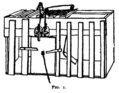
In the 1890s, the American psychologist Edward Thorndike put hungry cats into wooden cages with a door that opened from the inside. A loop of string, a lever or a latch released the door, and food waited outside. At first a cat scratched and pushed at everything. By chance it pulled the loop, the door opened, and it ate.
One of Thorndike's puzzle boxes, Figure 1 of his 1898 monograph on animal intelligence. Public domain, via Wikimedia Commons.
Thorndike timed each escape. Over many trials the time fell, slowly and unevenly, not in one flash of insight. The cat had not understood the latch. The action that led to food had simply become more likely.
In 1911 he stated the rule as the **law of effect**. Actions followed by satisfaction become more firmly connected to the situation. Actions followed by discomfort become less so.
> [!DEFINITION] Law of effect
> Thorndike's rule from animal learning. An action followed by a good result becomes more likely in the same situation, and one followed by a bad result becomes less likely.
That rule is the whole of reinforcement learning in one sentence. The rest of this part makes it precise. It also makes it work when the good result comes many steps after the action that earned it.
### The words of the field
Reinforcement learning uses a small set of words, and every method in this part fits them. Think of a video game. You are the **agent**, and the game is the **environment**. What is on the screen now is the **state**. The button you press is the **action**. The points you get are the **reward**.
> [!DEFINITION] Agent and environment
> The **agent** is the learner that chooses actions. The **environment** is everything outside it: a game, a robot's body and room, a market. The agent cannot change the environment's rules; it only chooses actions.
> [!DEFINITION] State, action and reward
> A **state** $$s$$ is the situation the agent is in. An **action** $$a$$ is one of the choices it can make there. A **reward** $$r$$ is a number the environment returns after each action: positive is good, negative is bad, and most steps give 0.
> [!DEFINITION] Policy
> The agent's way of choosing actions, written $$\pi(a \mid s)$$: the probability of taking action $$a$$ in state $$s$$. Learning in this field means finding a better policy.
Every method in this part fits this loop. Only the way the agent learns from the rewards changes.
The loop has one feature that makes it hard. The agent never sees the right action, only rewards, and a reward may arrive long after the action that caused it. A chess game is won or lost at move 60, but the mistake may have been move 12. Finding which earlier action deserves the credit is the **credit assignment problem**.
### Reward now, reward later
A reward now is worth more than the same reward later, partly because later is less certain. So the agent adds up future rewards, but shrinks each one by a factor for every step of waiting. The total is called the **return**.
$$
G_t = r_{t+1} + \gamma\, r_{t+2} + \gamma^2\, r_{t+3} + \dots = \sum_{k=0}^{\infty} \gamma^k\, r_{t+k+1}
$$
$$G_t$$ is the return from time step $$t$$. $$r_{t+1}$$ is the reward that arrives after the action at time $$t$$, $$r_{t+2}$$ the one after that, and so on. The **discount factor** $$\gamma$$ (gamma) is a number between 0 and 1. Each step of waiting multiplies a reward by one more $$\gamma$$.
> [!DEFINITION] Discount factor
> A number $$\gamma$$ between 0 and 1 that sets how much the agent cares about later rewards. With $$\gamma$$ near 0 it is short-sighted; with $$\gamma$$ near 1 it plans far ahead.
Take $$\gamma = 0.9$$ and three steps with rewards 0, 0 and 1. The return is $$0 + 0.9 \times 0 + 0.81 \times 1 = 0.81$$: the prize at the third step counts as 0.81 now. If the agent got a reward of 1 at every step forever, the return would be $$1 / (1 - 0.9) = 10$$. The discount keeps an endless sum finite.
## 1950s: Bellman's equation
### Dynamic programming
In the early 1950s, the mathematician Richard Bellman worked at the RAND Corporation on problems of planning over many stages. In 1957 he published the book *Dynamic Programming* and, the same year, the paper "A Markovian Decision Process". He framed decision-making as a world that moves from state to state, where each move depends only on the current state and the chosen action.
> [!DEFINITION] Markov decision process (MDP)
> A formal model of the loop. It has a set of states, a set of actions and the probability $$P(s' \mid s, a)$$ of reaching $$s'$$ after action $$a$$ in state $$s$$. It also has a reward for each step and a discount factor. "Markov" means the next state depends only on the current state and action, not on the earlier history.
Bellman's key idea is the **principle of optimality**. If the best route from Delhi to Mumbai passes through Pune, then its last part must be the best route from Pune to Mumbai. So you can solve a long problem backwards, one stage at a time, by reusing the answers to the smaller problems.
> [!DEFINITION] Dynamic programming
> A method that solves a big problem by breaking it into smaller ones that overlap, solving each smaller one once, and reusing its answer. In planning, the smaller problems are "what is the best I can do from here on?".
### The value of a state
The answer to "what is the best I can do from here on?" is a number, the **value** of a state.
> [!DEFINITION] Value function
> $$V^{\pi}(s)$$ is the expected return if the agent starts in state $$s$$ and then follows the policy $$\pi$$. A high value means "this is a good place to be, if I keep acting this way".
Our running example is a corridor of five cells. Cell 0 is a pit with a reward of $$-1$$ and cell 4 is a goal with a reward of $$+1$$. Reaching either one ends the episode. The agent starts in cell 2 and can step left or right. Every other step gives a reward of 0, and $$\gamma = 0.9$$.
The same cells have different values under different policies. A value is "how good it is to be here, if I keep acting this way". Numbers from our script.
The **Bellman expectation equation** links a state to its neighbours. The value of a state equals the reward of the next step plus the discounted value of where you land, averaged over what can happen.
$$
V^{\pi}(s) = \sum_{a} \pi(a \mid s) \sum_{s'} P(s' \mid s, a)\, \big[\, r + \gamma\, V^{\pi}(s') \,\big]
$$
Read it from the outside in. The first sum runs over the actions $$a$$, each weighted by how often the policy picks it, $$\pi(a \mid s)$$. The second sum runs over the next states $$s'$$, each weighted by its probability $$P(s' \mid s, a)$$. Inside the brackets, $$r$$ is the reward of that step and $$\gamma\, V^{\pi}(s')$$ is the discounted value of the next state.
Check it on cell 3 under a random policy that picks left or right half the time. Going right reaches the goal: reward 1, and the episode ends, so the next value is 0. Going left reaches cell 2, with reward 0, and $$V(2) = 0$$ by symmetry. So $$V(3) = 0.5 \times (1 + 0) + 0.5 \times (0 + 0.9 \times 0) = 0.5$$. Our script solves all three cells: $$-0.5$$, 0 and 0.5.
### The best policy and value iteration
The random policy is not very good. Bellman's second equation describes the best policy, by taking the best action instead of the average one.
$$
V^{*}(s) = \max_{a} \sum_{s'} P(s' \mid s, a)\, \big[\, r + \gamma\, V^{*}(s') \,\big]
$$
$$V^{*}$$ is the **optimal value function**: the value of each state when the agent acts as well as possible from then on. The $$\max_a$$ picks the action whose one-step look-ahead is largest. This is the **Bellman optimality equation**. Once you know $$V^{*}$$, the best policy is easy: in each state, take the action that achieves the max.
A backup looks one step ahead, adds the reward to the discounted value of the next cell, and keeps the best. Value iteration does this for every cell, again and again.
**Value iteration** solves the equation by starting from all zeros and applying it to every state again and again. On the corridor, the first sweep sets $$V(3) = 1$$, because the goal is one step away. The second sweep sets $$V(2) = 0.9$$, and the third sets $$V(1) = 0.81$$. From the fourth sweep on, nothing changes. The good news spread backwards from the goal, one cell per sweep.
> [!DEFINITION] Value iteration
> An algorithm that finds the optimal values by repeating the Bellman optimality update on every state until the values stop changing. Its close cousin is **policy iteration** (Ronald Howard, 1960). It alternates between computing the values of a policy and making the policy greedy with respect to those values.
There is a catch, and Bellman named it himself: the **curse of dimensionality**. Value iteration needs the full table of states and the probabilities $$P(s' \mid s, a)$$. Backgammon has more than $$10^{20}$$ positions and Go has far more. And in most real problems, nobody gives you $$P$$. The rest of this story is about learning from experience when the table is too large and the rules are unknown.
## 1951 to 1963: the first learning machines
### Samuel's checkers player
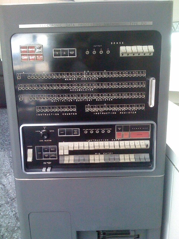
In the 1950s, Arthur Samuel at IBM wrote a program that played checkers on IBM's first commercial scientific computer, the IBM 701, and its successors. In 1959 he published "Some Studies in Machine Learning Using the Game of Checkers". He is often credited with making the term "machine learning" popular.
The operator's console of an IBM 701, on display at the Computer History Museum. Photo: Dan, CC BY 2.0, via Wikimedia Commons.
Samuel's program scored board positions with a weighted sum of features, such as the number of pieces on each side. It looked a few moves ahead and backed up the scores. Then it changed its weights so that the score of the current position moved toward the score that its look-ahead found. In effect, it learned to predict its own future judgement. That idea returned thirty years later as temporal-difference learning.
### MENACE, a learning machine made of matchboxes
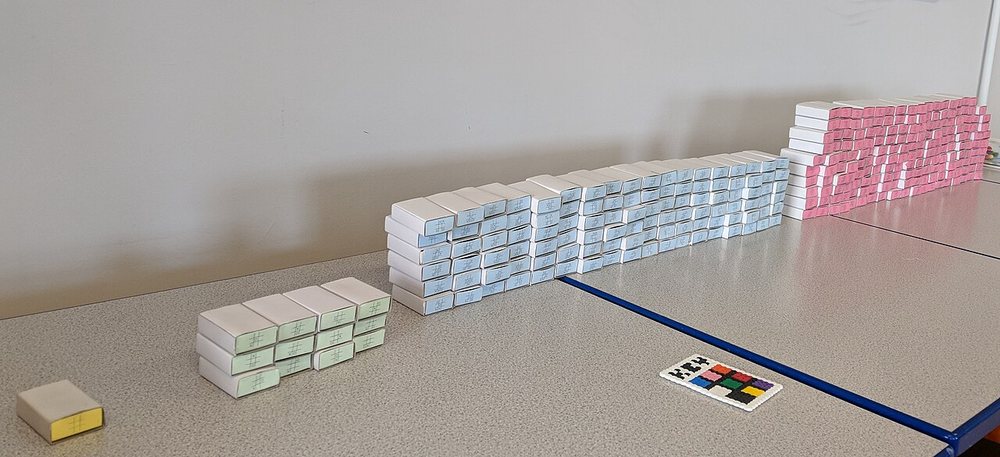
In 1961, the British researcher Donald Michie built a machine that learned noughts and crosses (tic-tac-toe) with no computer at all. MENACE, the Matchbox Educable Noughts And Crosses Engine, used about 304 matchboxes, one for each board position it could meet. Each box held coloured beads, one colour per possible move.
A modern rebuild of MENACE by Matthew Scroggs. Each matchbox stands for one board position. Photo: Matthew Scroggs, CC BY-SA 4.0, via Wikimedia Commons.
To move, you open the box for the current board and draw a bead at random. After a win, every box used in the game gets extra beads of the colour it played. After a loss, those beads are taken away. Winning moves become more likely and losing moves less likely, which is the law of effect built from cardboard. Each box holds a **policy** for one state, stored as a table of bead counts.
## Explore or exploit: the bandit problem
Suppose you have lived in a town for a month and have a favourite restaurant. Tonight you can go there again, which is safe, or try a new place, which might be better or worse. If you always go to your favourite, you never find out about the better one. If you always try new places, you waste most evenings. This is the **exploration-exploitation trade-off**.
> [!DEFINITION] Exploration and exploitation
> **Exploitation** means choosing the action that looks best so far. **Exploration** means trying other actions to learn more about them. An agent that only exploits can get stuck on a poor choice it happened to like early.
The cleanest version of the problem is a row of slot machines, each with an unknown chance of paying out. This is the **multi-armed bandit**, named after the "one-armed bandit" slot machine. William Thompson wrote about a version of it for medical trials in 1933, and Herbert Robbins framed the modern problem in 1952. There is only one state, so the whole difficulty is exploration.
The simplest strategy is **ε-greedy** (epsilon-greedy). Most of the time, pull the arm with the best average so far. With a small probability $$\varepsilon$$, pull a random arm instead. Our script tested two machines: arm A pays 1 with probability 0.4 and arm B with probability 0.6.
Arm A pays 1 with probability 0.4 and arm B with probability 0.6. Pure greed often locks onto the worse arm (it ends on arm B in only 57.9% of runs). A little exploration finds B every time. Numbers from our script.
Pure greed earned 0.5155 per pull on average, and it ended on the better arm B in only 57.9% of runs. With $$\varepsilon = 0.1$$, the agent earned 0.5815 per pull and picked arm B at the end of every one of the 2,000 runs. The best possible, always arm B, is 0.6. A little curiosity paid for itself many times over.
A smarter rule explores where it is most uncertain. Peter Auer, Nicolò Cesa-Bianchi and Paul Fischer analysed the **upper confidence bound** rule in 2002. It adds a bonus to each arm that shrinks as the arm is tried more often.
$$
a_t = \arg\max_{a} \left[\, Q(a) + c \sqrt{\frac{\ln t}{N(a)}} \,\right]
$$
$$Q(a)$$ is the average reward of arm $$a$$ so far, and $$N(a)$$ is how many times it has been pulled. $$t$$ is the total number of pulls. $$\ln$$ is the natural logarithm and $$c$$ sets the size of the bonus. "$$\arg\max_a$$" means "the arm that makes the bracket largest".
Take $$t = 100$$ and $$c = 1$$. Arm A has an average of 0.55 from 90 pulls and scores $$0.55 + 0.2262 = 0.7762$$. Arm B has an average of 0.40 from only 10 pulls and scores $$0.40 + 0.6786 = 1.0786$$. So the rule tries B again, because it knows too little about it.
## 1983 to 1992: learning from the difference
### The first actor and critic
In 1983, Andrew Barto, Richard Sutton and Charles Anderson trained a system to balance a pole on a moving cart. It had two parts: an "actor" that chose to push left or right, and a "critic" that learned to predict how well things were going. The only reward was a failure signal when the pole fell. The critic turned that rare signal into a running judgement of every moment, and the actor learned from the critic. This **actor-critic** design returns in every modern method.
### Temporal-difference learning, 1988
Think of a weather forecast for Saturday. On Monday it says 60% rain, on Tuesday 70%, on Wednesday 40%. You do not need to wait until Saturday to learn something. Each day's forecast is a better guess than the day before, so you can correct Monday's forecast using Tuesday's. In 1988, Richard Sutton published this idea as **temporal-difference (TD) learning**.
> [!PAPER] Sutton (1988), Learning to Predict by the Methods of Temporal Differences · Abstract · page 9
> [](/img/writings/history/h-sutton88.png)
>
> **What it says:** conventional methods assign credit "by means of the difference between predicted and actual outcomes". The new methods use "the difference between temporally successive predictions". Such methods had appeared in "Samuel's checker player" and elsewhere, but had "remained poorly understood".
>
> **What it means:**
>
> The old way waits for the final outcome and compares every prediction with it. TD compares each prediction with the very next one. That lets an agent learn during a game, not only at the end. Sutton also proved when it converges, which turned an old trick into a method.
The TD update for a value table fits in one line.
$$
V(s) \leftarrow V(s) + \alpha \big[\, r + \gamma\, V(s') - V(s) \,\big]
$$
The agent was in state $$s$$, got reward $$r$$, and landed in $$s'$$. The bracket is the **TD error**: what the agent now believes, $$r + \gamma V(s')$$, minus what it believed before, $$V(s)$$. The **learning rate** $$\alpha$$ (alpha), between 0 and 1, sets how far to move toward the new belief. The arrow means "replace with".
> [!DEFINITION] TD error
> The difference $$\delta = r + \gamma V(s') - V(s)$$ between the reward plus the estimated value of the next state, and the estimated value of the current state. It is positive when things went better than expected and negative when they went worse.
Use the corridor with every value at 0 and $$\alpha = 0.5$$. The agent steps from cell 3 into the goal and gets 1. The TD error is $$1 + 0.9 \times 0 - 0 = 1$$, so $$V(3)$$ becomes 0.5. In the next episode, it steps from cell 2 to cell 3 with reward 0. Now the error is $$0 + 0.9 \times 0.5 - 0 = 0.45$$, so $$V(2)$$ becomes 0.225. The good news travels backwards, one step per visit, with no model of the world at all.
In 1997, Wolfram Schultz, Peter Dayan and Read Montague reported that dopamine neurons in monkeys fire in a pattern that matches the TD error. A surprise reward makes them fire, and a reward that was fully expected does not. The equation written for machines seemed to describe the brain too.
### Q-learning, 1989
TD learning tells you how good a state is, but to act you need to know how good each action is. In his 1989 PhD thesis at Cambridge, Christopher Watkins learned the value of each state and action pair instead, written $$Q(s, a)$$. In 1992, Watkins and Peter Dayan proved that the method converges to the best values if every pair is tried often enough.
> [!DEFINITION] Action value (Q-value)
> $$Q(s, a)$$ is the expected return if the agent takes action $$a$$ in state $$s$$ and then acts well. The best action in a state is the one with the highest Q-value. "Q" is for quality.
$$
Q(s, a) \leftarrow Q(s, a) + \alpha \big[\, r + \gamma \max_{a'} Q(s', a') - Q(s, a) \,\big]
$$
This is the TD update with one change. The target uses $$\max_{a'} Q(s', a')$$, the value of the best action in the next state, whatever action the agent will really take. So the agent can explore at random and still learn the values of the best policy. Methods with this property are called **off-policy**.
> [!DEFINITION] Off-policy learning
> Learning about one policy (usually the best one) from actions chosen by a different policy (for example an exploring one). Q-learning is off-policy. **SARSA** (Gavin Rummery and Mahesan Niranjan, 1994) is the on-policy version: its target uses the action the agent really takes next.
A Q-table holds one number per state and action. The update moves one entry part of the way toward "reward now plus the best value next". These are the third and fourth updates of our run.
Our script ran Q-learning on the corridor for 500 episodes with $$\alpha = 0.5$$ and $$\varepsilon = 0.2$$. In the first episode the agent wandered into the pit, so $$Q(1, \text{left})$$ became $$-0.5$$. In the second it reached the goal from cell 3, so $$Q(3, \text{right})$$ became 0.5. In the third, the update in the figure set $$Q(2, \text{right})$$ to 0.225. After 500 episodes, every entry was within 0.0078 of the exact values from value iteration, and the greedy policy was "right" in every cell.
### TD-Gammon, 1992
Backgammon has dice, so the same move can lead to many positions, and the number of positions is enormous. At IBM, Gerald Tesauro combined TD learning with a neural network that read a board and predicted the chance of winning. The program played against itself, starting from random weights, and used TD updates after every move. He called it **TD-Gammon**.
> [!DEFINITION] Self-play
> Training an agent by letting it play games against copies of itself. As the agent improves, so does its opponent, so the difficulty keeps rising.
The result surprised many people. In his 1995 article, Tesauro reported that version 2.1 reached near-parity with the former world champion Bill Robertie in a 40-game test. Robertie judged that it played "at a strong master level". A network with no expert knowledge had learned an expert game from its own play. It was also the first big success of a neural network inside reinforcement learning.
## 1992 to 2000: pushing the policy directly
### REINFORCE, 1992
Values are one road to a good policy. A second road skips values and adjusts the policy itself. Think of a basketball player who shoots many times. Each time the ball goes in, they make that motion a little more likely; each miss makes it a little less likely. In 1992, Ronald Williams published this idea for neural networks as **REINFORCE**.
> [!DEFINITION] Policy gradient
> A method that represents the policy with parameters $$\theta$$, for example the weights of a network. It changes them by gradient ascent on the expected return, so actions that led to high returns become more likely.
$$
\nabla_{\theta} J(\theta) = \mathbb{E}_{\pi_\theta} \big[\, G_t \, \nabla_{\theta} \log \pi_{\theta}(a_t \mid s_t) \,\big]
$$
$$J(\theta)$$ is the expected return of the policy with parameters $$\theta$$. $$\nabla_\theta$$ means "the gradient with respect to $$\theta$$": the direction in parameter space that increases a quantity fastest. $$\log \pi_\theta(a_t \mid s_t)$$ is the log-probability of the action the agent took. $$G_t$$ is the return that followed. $$\mathbb{E}_{\pi_\theta}$$ means "on average over episodes played with this policy".
Read it as an instruction. Find the direction that makes the action you took more likely, and step that way in proportion to how good the outcome was. A big return gives a big push. A return of 0 gives no push at all.
Take the two slot machines again, with a policy that picks an arm by softmax over two numbers $$\theta = (\theta_A, \theta_B)$$. Both start at 0, so each arm has probability 0.5. The agent pulls B and gets a reward of 1. The gradient of $$\log \pi(B)$$ is $$(-0.5, 0.5)$$. With a learning rate of 0.1, $$\theta$$ becomes $$(-0.05, 0.05)$$, and the probability of B rises from 0.5 to 0.525.
### The baseline
REINFORCE has a weakness: its pushes are noisy. If every reward is positive, every action gets pushed up, and only the sizes of the pushes differ. The fix is to subtract a **baseline** $$b$$, such as the average reward so far, and use $$G_t - b$$ in place of $$G_t$$. Williams showed that this keeps the gradient correct on average.
With $$b = 0.5$$, a pull of B with reward 1 now gives a push of $$0.5$$ in place of 1, and $$\pi(B)$$ moves to 0.5125. A pull of A with reward 0 gives $$0 - 0.5 = -0.5$$: A becomes less likely, and B rises to the same 0.5125. A bad result now teaches as much as a good one. In our 500 simulated runs, the baseline cut the variance of the update from 0.1140 to 0.0711. Both versions ended with a probability for B of about 0.93 (0.929 and 0.934).
> [!DEFINITION] Variance
> A measure of how much a quantity jumps around its average. A gradient estimate with high variance points in a different direction each time, so learning needs smaller steps and more samples.
### The policy gradient theorem and the advantage
In 1999, Richard Sutton, David McAllester, Satinder Singh and Yishay Mansour proved the **policy gradient theorem**. It shows that the return $$G_t$$ in the formula can be replaced by the action value $$Q^{\pi}(s, a)$$, even when a neural network approximates the policy. With a state value as the baseline, the push becomes the **advantage**.
> [!DEFINITION] Advantage
> $$A(s, a) = Q(s, a) - V(s)$$: how much better action $$a$$ is than the average action in state $$s$$. A positive advantage means "better than usual". It is the signal that almost every modern policy method uses.
A **critic** can estimate the advantage from a single step, with the TD error from before.
$$
A(s, a) \approx r + \gamma\, V(s') - V(s)
$$
Say the critic believes $$V(s) = 0.5$$ and $$V(s') = 0.81$$, and the step gave reward 0. The advantage is $$0 + 0.9 \times 0.81 - 0.5 = 0.229$$: this action was a bit better than the critic expected, so the actor makes it more likely. The actor learns the policy, and the critic learns the values that judge it. It is the 1983 design with a theory behind it.
The critic replaces the noisy total return of REINFORCE with a one-step estimate. That lowers the variance, at the cost of some bias from the critic's own mistakes.
In 1998, Sutton and Barto published the textbook *Reinforcement Learning: An Introduction*, which collected these ideas. Its second edition came out in 2018. By 2000 the theory was mostly in place. What was missing was a way to make it work on big, messy problems.
## 2013 to 2015: deep Q-networks play Atari
### From tables to networks
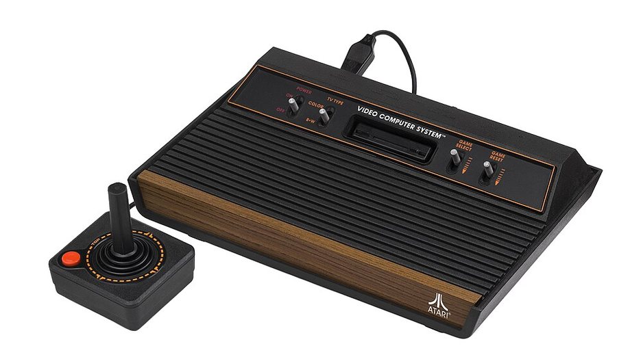
The corridor has six Q-values. An Atari game screen has 210 by 160 pixels with 128 possible colours, far too many states for a table. The obvious idea is to let a neural network compute $$Q(s, a)$$ from the pixels. For years it worked badly: training often became unstable and the values blew up.
> [!DEFINITION] Function approximation
> Using a function with parameters, such as a neural network, to estimate values or a policy. It replaces a table with one entry per state. It lets the agent handle states it has never seen, but learning becomes less stable.
An Atari 2600 console from 1977. Its games became the standard test for reinforcement learning from pixels. Photo: Evan-Amos, public domain, via Wikimedia Commons.
In December 2013, Volodymyr Mnih and colleagues at DeepMind, a London start-up, posted "Playing Atari with Deep Reinforcement Learning". Their deep Q-network (**DQN**) played seven Atari games from raw pixels. In February 2015, a longer paper in *Nature*, "Human-level control through deep reinforcement learning", tested the same network on 49 games. It used the same architecture and settings for every game, and its scores were compared with a professional human games tester.
> [!PAPER] Mnih et al. (2015), Human-level control through deep reinforcement learning · Figure 1 · page 2
> [](/img/writings/history/h-dqn-fig.png)
>
> **What it says:** a "schematic illustration of the convolutional neural network". The input is "an 84 × 84 × 4 image", followed by "three convolutional layers" and "two fully connected layers with a single output for each valid action".
>
> **What it means:**
>
> The network sees the last four frames, so it can tell which way the ball moves. It outputs one Q-value per joystick action, so a single forward pass scores every action at once. The image goes in at the left; the right column of buttons is the Q-table, now computed instead of stored.
### Two fixes that made it stable
The Nature paper names the two key ideas. The first is **experience replay**, from Long-Ji Lin's work in 1992. The agent stores its recent steps, the last 1 million frames, and trains on random samples from that memory. Consecutive frames of a game are almost the same. Training on them in order is like studying one page of a book a thousand times.
> [!DEFINITION] Experience replay
> A memory of past steps $$(s, a, r, s')$$ that the agent samples from at random during training. It breaks the correlation between consecutive steps and lets each step be reused many times.
The second is a **target network**: a frozen copy of the Q-network that computes the targets, updated only every so often. Without it, every update changes the target too, like a dog chasing its own tail.
$$
L(\theta) = \mathbb{E}_{(s, a, r, s') \sim \mathcal{D}} \Big[ \big(\, r + \gamma \max_{a'} Q(s', a'; \theta^{-}) - Q(s, a; \theta) \,\big)^2 \Big]
$$
$$\theta$$ are the weights of the Q-network and $$\theta^{-}$$ the weights of the frozen copy. $$\mathcal{D}$$ is the replay memory, and $$\sim$$ means "sampled from". The term in the large brackets is the TD error of Q-learning, squared. Training lowers this loss by gradient descent on $$\theta$$ only.
Say the frozen network scores the three actions in the next state as 0.6, 1.4 and 0.9. The reward is 0.5, and the online network says $$Q(s, a) = 1.2$$. The target is $$0.5 + 0.9 \times 1.4 = 1.76$$. The loss is $$(1.76 - 1.2)^2 = 0.3136$$, and the gradient pulls $$Q(s, a)$$ up toward 1.76.
The two fixes of DQN. The replay buffer breaks the chain of similar frames by training on random old steps. The frozen target network keeps the target from moving at every step. The 1-million-frame memory is the size the 2015 Nature paper reports.
In 2014 Google bought DeepMind, and the next years brought a stream of fixes. **Double DQN** (Hado van Hasselt and colleagues, 2015) fixed the habit of overestimating values. Prioritised replay, the duelling network and their combination, **Rainbow**, raised scores further. In 2020 DeepMind's **Agent57** beat the standard human benchmark on all 57 Atari games.
## 2015 to 2017: stable policy gradients
Q-learning picks the action with the highest value, which works for a joystick with 18 buttons. A robot arm has continuous joint angles, and there is no list of actions to take a max over. Policy gradients handle such actions naturally, but they had a stability problem. One step too large could wreck a good policy, and the agent then collected bad data from the wrecked policy.
### A3C and TRPO
In 2016, Mnih and colleagues published **A3C**, the asynchronous advantage actor-critic. It ran many copies of the agent in parallel on the cores of one CPU, each in its own copy of the game. All of them updated one shared network. The paper reports that it beat the previous best on Atari while training for half the time, on a CPU in place of a GPU.
In 2015, John Schulman, Sergey Levine, Pieter Abbeel and colleagues at Berkeley published **trust region policy optimisation** (TRPO). Its rule: improve the policy, but keep the new policy within a fixed KL divergence of the old one. KL divergence measures how different two probability distributions are, and Part 1 met it briefly. TRPO was stable, but it needed second-order maths that was slow and hard to implement.
> [!DEFINITION] Trust region
> A limit on how far one update may move the policy, measured as a distance between the old and new action probabilities. Inside the region, the local estimate of the improvement can be trusted.
### PPO, 2017
In July 2017, Schulman and colleagues, now at OpenAI, published **proximal policy optimisation** (PPO). It reaches the same goal with a simple trick. First compute the **probability ratio**: how much more or less likely the new policy makes the action than the old one did.
$$
r_t(\theta) = \frac{\pi_{\theta}(a_t \mid s_t)}{\pi_{\theta_\text{old}}(a_t \mid s_t)}
$$
If the old policy gave an action probability 0.20 and the new one gives 0.30, the ratio is $$0.30 / 0.20 = 1.5$$. A ratio of 1 means no change. PPO then limits how much a single batch of data can push this ratio.
$$
L^{\text{CLIP}}(\theta) = \mathbb{E}_t \Big[ \min\big(\, r_t(\theta)\, \hat{A}_t,\;\; \text{clip}\big(r_t(\theta),\, 1 - \epsilon,\, 1 + \epsilon\big)\, \hat{A}_t \,\big) \Big]
$$
$$\hat{A}_t$$ is the estimated advantage of the action at step $$t$$. $$\text{clip}(r, 1 - \epsilon, 1 + \epsilon)$$ forces the ratio into the range $$[1 - \epsilon, 1 + \epsilon]$$, and $$\epsilon$$ (epsilon) is usually 0.2. The $$\min$$ takes the smaller of the clipped and the unclipped term. The agent maximises this objective.
> [!PAPER] Schulman et al. (2017), Proximal Policy Optimization Algorithms · §3 · page 3
> [](/img/writings/history/h-ppo-clip.png)
>
> **What it says:** clipping the probability ratio "removes the incentive for moving $$r_t$$ outside of the interval $$[1-\epsilon, 1+\epsilon]$$". Taking the minimum makes the objective "a lower bound (i.e., a pessimistic bound) on the unclipped objective".
>
> **What it means:**
>
> "Pessimistic" is the key word. When a change would help, PPO counts the gain only up to the clip, so there is no reason to move further. When a change would hurt, PPO counts the full loss. The policy improves in small, safe steps, and the same batch of data can be reused for several epochs.
Our script evaluates one term for a few ratios. For a good action ($$\hat{A} = +1$$) at $$r = 1.5$$, the unclipped term is 1.5 but the objective is only 1.2, the clip. At $$r = 0.5$$, nothing is clipped: the objective is 0.5, and the gradient still pushes the probability back up. For a bad action ($$\hat{A} = -1$$) at $$r = 1.5$$, the objective is the full $$-1.5$$, so the policy is pulled back hard.
The dots are the rows of our script: at r = 1.5 a good action scores 1.2, not 1.5, and a bad action scores −1.5, not −1.2. The clip limits gains, never losses.
> [!PAPER] Schulman et al. (2017), Proximal Policy Optimization Algorithms · Figure 1 · page 3
> [](/img/writings/history/h-ppo-fig.png)
>
> **What it says:** the plots show "one term (i.e., a single timestep) of the surrogate function $$L^{CLIP}$$ as a function of the probability ratio $$r$$, for positive advantages (left) and negative advantages (right)". The red circle is the start, $$r = 1$$.
>
> **What it means:**
>
> These are the same shapes as our chart, drawn by the authors. The flat parts are where the gradient is zero, so the update stops there. The paper says PPO is "much simpler to implement" than TRPO, and this one picture is most of the reason. Five years later, PPO was the algorithm in the third stage of RLHF.
PPO usually estimates advantages with **generalised advantage estimation** (GAE), from Schulman and colleagues in 2015. GAE mixes one-step, two-step and longer TD estimates, trading a little bias for much less variance. For continuous control, **soft actor-critic** (Tuomas Haarnoja and colleagues, 2018) became a strong alternative. It rewards the policy for staying random where it can, which helps exploration.
## 2016 to 2020: self-play and search
### AlphaGo
Part 1 told how AlphaGo beat Lee Sedol in March 2016. Its *Nature* paper, published that January, shows how reinforcement learning fit inside it. A policy network first learned to predict expert moves from human games. Policy gradient learning then improved it by self-play, and a value network learned to predict the winner from self-play positions. A tree search used both networks to look ahead.
> [!PAPER] Silver et al. (2016), Mastering the game of Go with deep neural networks and tree search · Figure 1 · page 485
> [](/img/writings/history/h-alphago-fig.png)
>
> **What it says:** the "neural network training pipeline and architecture". The supervised policy network is trained "to predict human expert moves". The RL policy network "is then improved by policy gradient learning to maximize the outcome". A value network "is trained by regression to predict the expected outcome".
>
> **What it means:**
>
> Read panel a from left to right: imitation first, then reinforcement, then a judge. The arrow marked "Policy gradient" is REINFORCE at the scale of a Go board. Panel b shows the two networks: one outputs a probability map over moves, the other a single number. The same paper reports a 99.8% win rate against other Go programs and a 5 to 0 win over the European champion Fan Hui.
### AlphaGo Zero: no human games
In October 2017, David Silver and colleagues published "Mastering the Game of Go without Human Knowledge". AlphaGo Zero dropped the human games, the hand-made input features and the separate networks. One network, with a policy output and a value output, learned only from self-play. The search did the teaching.
> [!PAPER] Silver et al. (2017), Mastering the Game of Go without Human Knowledge · Abstract · page 1
> [](/img/writings/history/h-agz-abs.png)
>
> **What it says:** the algorithm is "based solely on reinforcement learning, without human data, guidance, or domain knowledge beyond game rules". "AlphaGo becomes its own teacher". Starting "tabula rasa", it won "100-0 against the previously published, champion-defeating AlphaGo".
>
> **What it means:**
>
> "Tabula rasa" is Latin for a blank slate. Human games had been a crutch, and also a ceiling. The paper reports that training ran for about three days and produced 4.9 million self-play games. AlphaGo Zero passed the version that beat Lee Sedol after 36 hours.
### AlphaZero: one algorithm, three games
In December 2017, the same team posted **AlphaZero**. It used the AlphaGo Zero method, nearly unchanged, for chess, shogi (Japanese chess) and Go.
> [!PAPER] Silver et al. (2017), Mastering Chess and Shogi by Self-Play with a General Reinforcement Learning Algorithm · Abstract · page 1
> [](/img/writings/history/h-alphazero.png)
>
> **What it says:** "Starting from random play, and given no domain knowledge except the game rules, AlphaZero achieved within 24 hours a superhuman level of play in the games of chess and shogi (Japanese chess) as well as Go". It "convincingly defeated a world-champion program in each case".
>
> **What it means:**
>
> Deep Blue's chess knowledge took engineers and grandmasters years to write. AlphaZero learned chess in less than a day from the rules alone. In chess its opponent was Stockfish, the champion engine of 2016. The same code, with no game-specific tricks, worked in all three games.
AlphaZero's search is a **Monte Carlo tree search** (MCTS). It grows a tree of possible futures from the current position, one path per **simulation**. Each simulation picks its next move with the **PUCT** rule.
> [!DEFINITION] Monte Carlo tree search (MCTS)
> A search that grows a tree of possible moves step by step. Each simulation walks down the tree, picking moves that look promising or are still unexplored. It scores the new position and passes the score back up the path. Moves that are visited most are the best ones.
$$
a = \arg\max_{a} \left[\, Q(s, a) + c_{\text{puct}}\, P(s, a)\, \frac{\sqrt{\sum_b N(s, b)}}{1 + N(s, a)} \,\right]
$$
$$Q(s, a)$$ is the average value found so far below move $$a$$. $$P(s, a)$$ is the network's prior probability for the move. $$N(s, a)$$ counts how often the search has tried the move, and $$\sum_b N(s, b)$$ counts all visits to this position. The second term is an exploration bonus, like the bonus in the bandit rule. It is large for moves the network likes but the search has rarely tried, and $$c_{\text{puct}}$$ sets its weight.
Take three moves and $$c_{\text{puct}} = 1.5$$, with 12 visits so far. Move a has $$Q = 0.50$$, prior 0.6 and 10 visits, for a score of $$0.50 + 0.2834 = 0.7834$$. Move b has $$Q = 0.40$$, prior 0.3 and 2 visits, for $$0.40 + 0.5196 = 0.9196$$. Move c has never been tried and scores 0.5196. The search tries move b next: its value is lower, but it is under-explored.
Policy improvement and policy evaluation, the two halves of Bellman's dynamic programming, here done by a search and a network. 800 simulations per move is the setting reported for AlphaZero.
After the search, the visit counts give a new, better policy $$\pi$$, and the end of the game gives the result $$z$$. The network learns both with one loss.
$$
\ell = (z - v)^2 - \boldsymbol{\pi}^{\top} \log \mathbf{p} + c\, \lVert \theta \rVert^2
$$
$$v$$ is the network's value prediction and $$z$$ the real result, $$+1$$ for a win and $$-1$$ for a loss. So the first term is a squared error. $$\mathbf{p}$$ is the network's move probabilities and $$\boldsymbol{\pi}$$ the search's. The second term is the cross-entropy between them, which pulls the network toward the search. The last term is **L2 regularisation**: a small penalty on large weights, with strength $$c$$, which keeps the network from overfitting.
Say the game was won ($$z = 1$$) and the network predicted $$v = 0.6$$: the value term is $$(1 - 0.6)^2 = 0.16$$. The search visited three moves in the proportions 0.7, 0.2 and 0.1, and the network gave them 0.5, 0.3 and 0.2. The policy term is $$-(0.7 \ln 0.5 + 0.2 \ln 0.3 + 0.1 \ln 0.2) = 0.8869$$. The total, before the weight penalty, is 1.0469. Each training step lowers it a little.
### MuZero: learning the rules too
AlphaZero needed the rules to run its search. In November 2019, Julian Schrittwieser and colleagues posted **MuZero**, which learns a model of the game and plans inside it.
> [!DEFINITION] Model-based reinforcement learning
> Reinforcement learning in which the agent learns, or is given, a model that predicts what happens after an action. It can then plan by imagining futures with the model, in place of trying them all in the real world.
> [!PAPER] Schrittwieser et al. (2019), Mastering Atari, Go, Chess and Shogi by Planning with a Learned Model · Figure 1 · page 3
> [](/img/writings/history/h-muzero-fig.png)
>
> **What it says:** "Planning, acting, and training with a learned model." The model has "three connected components for representation, dynamics and prediction". The dynamics function $$g$$ "produces an immediate reward $$r^k$$ and a new hidden state $$s^k$$".
>
> **What it means:**
>
> In panel A, $$h$$ turns the real board into a hidden state, $$g$$ imagines one move ahead, and $$f$$ gives a policy and a value. The hidden states never have to look like a board; they only have to predict rewards, values and policies well. The abstract reports that MuZero matched AlphaZero in Go, chess and shogi "without any knowledge of the game rules", and set a new best on 57 Atari games.
### Teams, fog and real time
Board games show the whole position to both players. Video games add hidden information, real time and teams. In April 2019, **OpenAI Five** beat OG, the world champion team at the five-player game Dota 2. The paper says it trained for 10 months, on batches of about 2 million frames every 2 seconds. Its learning algorithm was PPO, at a very large scale.
In October 2019, DeepMind's **AlphaStar** reached Grandmaster level in StarCraft II, playing on the public game server under limits set with professional players. The *Nature* paper reports a rank above 99.8% of officially ranked human players. It combined imitation of human games with a "league" of agents that trained against each other, so no single strategy could dominate.
## Robots: from simulation to the real world
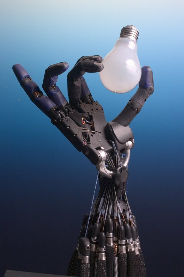
Games are cheap: you can play millions of them. A real robot breaks, needs a person to reset it, and runs only in real time. So most robot learning happens in a physics simulator first. The trouble is the **reality gap**. A policy that is perfect in simulation often fails on the real machine, because the simulator gets friction, weight and delay slightly wrong.
A Shadow Dexterous Hand, the robot hand OpenAI later trained in simulation. Photo: Richard Greenhill and Hugo Elias of the Shadow Robot Company, CC BY-SA 3.0, via Wikimedia Commons.
> [!PAPER] OpenAI et al. (2018), Learning Dexterous In-Hand Manipulation · Abstract · page 1
> [](/img/writings/history/h-dactyl.png)
>
> **What it says:** training happens "in a simulated environment in which we randomize many of the physical properties of the system like friction coefficients and an object's appearance". The policies "transfer to the physical robot despite being trained entirely in simulation".
>
> **What it means:**
>
> The trick is called **domain randomisation**. If the policy has practised in thousands of slightly different simulated worlds, the real world looks like just one more of them. The paper also says the same distributed RL system trained OpenAI Five. In 2019, OpenAI used a larger version of the method to solve a Rubik's Cube with the same hand.
> [!DEFINITION] Sim-to-real transfer
> Training a policy in a simulator and then running it on a real robot. Methods such as domain randomisation vary the simulator's physics during training so that the policy works across the range that includes the real world.
## Beyond games
The same tools began to work on problems with a clear score but no opponent. In 2022, DeepMind's **AlphaTensor** treated the search for a matrix multiplication method as a one-player game. It found a method for 4 by 4 matrices in arithmetic modulo 2 with 47 multiplications. The best method known before, from Strassen's 1969 work, needed 49.
In July 2024, **AlphaProof** used reinforcement learning to prove maths problems in Lean, a language in which a computer checks every step of a proof. Together with AlphaGeometry 2, it solved four of the six problems at the International Mathematical Olympiad, 28 points, the standard of a silver medal. A proof checker gives a reward that cannot be fooled, an idea that returns in Part 4.
## The bitter lesson
In March 2019, Richard Sutton published a short essay called "The Bitter Lesson". Its first sentence sums up seventy years: "The biggest lesson that can be read from 70 years of AI research is that general methods that leverage computation are ultimately the most effective, and by a large margin." The two methods that scale, he argued, are search and learning.
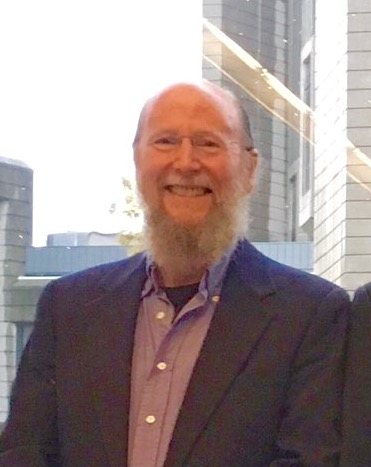
Richard Sutton in 2016. Photo: Steve Jurvetson, CC BY 2.0, via Wikimedia Commons.
The lesson is bitter because researchers like to build their own knowledge into a system, and that works in the short run. Deep Blue used grandmasters' chess knowledge; AlphaZero used none and won. TD-Gammon and AlphaGo Zero point the same way. The essay is now quoted far beyond reinforcement learning, often about language models.
On 5 March 2025, the Association for Computing Machinery named Andrew Barto and Richard Sutton the winners of the 2024 Turing Award, computing's highest prize. The ACM credited them with the conceptual and algorithmic foundations of reinforcement learning, from the papers of the 1980s on. Thorndike's rule had become a branch of computer science with a Turing Award.
## What reinforcement learning hands to language models
Every success in this part had a clear reward: the game's score, a win or a loss, a cube that is solved or not. Language has no score. Nobody can write a function that returns "how helpful was this answer?". That is why, for years, reinforcement learning and language models met only at the edges.
The bridge came from a simple idea: if you cannot write the reward, learn it from people's choices. In 2017, a team from OpenAI and DeepMind trained agents from human comparisons of short video clips. From 2019 to 2022, OpenAI applied the idea to text, and the training algorithm was PPO. Today, the newest reasoning models also learn from rewards that a program can check, like a proof checker or a unit test. [Part 4](https://ishwarj.com/writings/how-models-are-trained-today/) tells that story, from the first preference-trained summaries to the reasoning models of 2026.
| Step | What it fixed | What it left open |
|---|---|---|
| Law of effect (1911) | Learning from good and bad results | No account of delayed results |
| Bellman equation, MDPs (1957) | Exact planning over many steps | Needs the full model; too many states |
| Samuel, MENACE (1959, 1961) | Machines that improve by playing | Small games, hand-made features |
| Bandits, ε-greedy, UCB | A principled answer to exploration | Only one state |
| TD learning, Q-learning (1988, 1989) | Learning values from experience, no model | Tables; one entry per state |
| TD-Gammon (1992) | A neural network as the value function | Unstable on most other problems |
| REINFORCE, policy gradient theorem (1992, 1999) | Learning a policy directly; continuous actions | High variance |
| DQN (2013, 2015) | Stable deep Q-learning from pixels | Discrete actions; many frames needed |
| TRPO, PPO (2015, 2017) | Stable, simple policy updates | Still needs a reward function |
| AlphaGo to MuZero (2016 to 2019) | Superhuman play by self-play and search | Needs a simulator or a learned model |
| Sim-to-real (2018, 2019) | Robot skills learned in simulation | The reality gap; costly compute |
| Learned rewards (2017 onward, Part 4) | Rewards for goals nobody can write down | Reward hacking; human cost |
> [!TAKEAWAYS]
> - Reinforcement learning is Thorndike's law of effect made precise: actions followed by reward become more likely.
> - Bellman's equation says that a state's value is the reward now plus the discounted value of what follows. Nearly every method solves it in some cheaper way.
> - TD learning and Q-learning learn values from experience one step at a time, by correcting each prediction with the next one.
> - Policy gradients push the probabilities of good actions up directly; baselines and advantages cut their noise, and PPO's clip keeps each step safe.
> - DQN made deep networks work as value functions with experience replay and a target network.
> - AlphaGo Zero and AlphaZero learned superhuman play from the rules alone, by self-play and tree search; MuZero learned the rules too.
> - PPO and the idea of a learned reward carried this line into the training of language models.
Key papers: [Sutton 1988](https://doi.org/10.1007/BF00115009), [Watkins and Dayan 1992](https://doi.org/10.1007/BF00992698), [Williams 1992](https://doi.org/10.1007/BF00992696), [DQN 2015](https://doi.org/10.1038/nature14236), [PPO 2017](https://arxiv.org/abs/1707.06347), [AlphaGo Zero 2017](https://doi.org/10.1038/nature24270), [MuZero 2019](https://arxiv.org/abs/1911.08265), [Sutton and Barto's book](http://incompleteideas.net/book/the-book-2nd.html).
Next: [Part 4, From RLHF to Reasoning](https://ishwarj.com/writings/how-models-are-trained-today/), how these methods became the way language models are trained today.