# Inside a Modern Language Model: Data, Scale and Architecture
Author: Ishwar Jangid
Canonical URL: https://ishwarj.com/writings/inside-a-modern-language-model/
Updated: 2026-10-22
Source: https://github.com/ishwar6/ishwar-books/blob/main/content/writings/inside-a-modern-language-model.md
In 2024, Meta trained a language model with 405 billion parameters on 15.6 trillion tokens of text. The run used up to 16,384 GPUs. In one 54-day stretch of it, the job stopped 466 times, most often because a piece of hardware failed. Each time, the system loaded the last saved copy of the model and carried on.
At the end there was a file of numbers that could continue almost any text. No chat training had happened yet. That file is the **base model**, and it is the subject of this part. What goes into it? How big should it be? What does each layer look like inside, and what does it cost to make?
This is Part 5 of How AI Got Here. [Part 1](https://ishwarj.com/writings/from-neuron-to-opus/) told the story of neural networks up to the Transformer and the first scaling laws. [Part 2](https://ishwarj.com/writings/classical-machine-learning/) covered classical machine learning, and [Part 3](https://ishwarj.com/writings/reinforcement-learning-history/) covered reinforcement learning. [Part 4](https://ishwarj.com/writings/how-models-are-trained-today/) showed how a base model becomes an assistant. This part goes back one step and opens the base model itself, as it is built in October 2026.
> [!TIP] The whole idea in one minute
> A base model learns one thing: to predict the next token. How well it learns depends on three numbers: its size, its data and its compute. **Scaling laws** say how to split a budget between them. **Chinchilla** showed in 2022 that models were too big for their data. Today small models are trained on far more data than that rule says, because they are cheaper to run.
>
> The data is mostly the public web, filtered hard and deduplicated, plus code, maths and some text written by other models. The layer is still the 2017 Transformer, with new parts: **RMSNorm**, **SwiGLU**, **RoPE** and shared keys and values. Many frontier models are **mixtures of experts**, where each token uses only a small part of the network. Training spreads one model over thousands of chips, in 16-bit or even 8-bit numbers.
The core of the 2017 design is still there. Most changes after 2020 make the same model cheaper to train, cheaper to serve, or able to read longer inputs.
## What pre-training optimises
### One loss, read off every token
Part 1 introduced the **next-token loss**. The model reads a text, and at every position it gives a probability to each possible next token. The loss is the negative log of the probability it gave to the token that really came next. Averaged over trillions of positions, that one number is the whole goal of pre-training.
> [!DEFINITION] Cross-entropy loss
> The average, over all positions, of $$-\log p$$, where $$p$$ is the probability the model gave to the true next token. It is measured in nats when the natural logarithm is used. Lower is better.
The loss is hard to feel, so people often turn it into **perplexity**. Think of a quiz where the model must guess the next word. A perplexity of 7 means the model is as unsure as if it had to pick fairly between 7 equal choices at every step.
$$
\text{PPL} = \exp\!\Big( -\frac{1}{T} \sum_{t=1}^{T} \log p_\theta(x_t \mid x_{ [!DEFINITION] Perplexity
> The exponential of the average cross-entropy loss. It reads as "the number of equally likely choices the model is torn between". A model that guesses at random over $$V$$ tokens has perplexity $$V$$.
Our script gives the scale. A new model that guesses at random over a vocabulary of 128,000 tokens has a loss of $$\ln 128{,}000 = 11.76$$ and a perplexity of 128,000. A loss of 4.0 is a perplexity of 54.60, and a loss of 2.0 is 7.39. A single token with probability 0.9 costs 0.105; one with probability 0.01 costs 4.605.
> [!WARNING] Loss is not ability
> Two losses can be compared only on the same test text with the same tokenizer. A tokenizer with longer tokens makes each prediction harder, so the loss per token rises even if the model is better. Labs report losses for planning, and benchmarks for ability.
## Scaling laws: how big, how long
### Counting the compute
A **FLOP** is one floating-point operation, such as one multiply or one add. Training cost is counted in FLOPs, and there is a famous shortcut for it.
> [!DEFINITION] FLOP
> One floating-point operation, such as $$a \times b$$ or $$a + b$$ on real numbers. Training budgets are given as a total count of FLOPs; chip speed is given in FLOPs per second.
$$
C \approx 6 N D
$$
$$C$$ is the total training compute in FLOPs, $$N$$ is the number of parameters and $$D$$ is the number of training tokens. Each parameter takes part in one multiply and one add for each token on the forward pass, which is 2 FLOPs. The backward pass costs about twice the forward pass, which adds 4. So every parameter costs about 6 FLOPs per token.
A model with 1 billion parameters trained on 20 billion tokens costs $$6 \times 10^9 \times 2 \times 10^{10} = 1.2 \times 10^{20}$$ FLOPs. The rule leaves out the attention scores, which matter only for long texts. Jared Kaplan and colleagues used it in their 2020 paper, and almost every lab uses it today.
Here are some real runs, from our script:
| Model | Parameters $$N$$ | Tokens $$D$$ | $$6ND$$ (FLOPs) | Tokens per parameter |
|---|---|---|---|---|
| GPT-3 (2020) | 175B | 300B | $$3.15 \times 10^{23}$$ | 1.7 |
| Gopher (2021) | 280B | 300B | $$5.04 \times 10^{23}$$ | 1.1 |
| Chinchilla (2022) | 70B | 1.4T | $$5.88 \times 10^{23}$$ | 20 |
| Llama 3 8B (2024) | 8B | 15T | $$7.2 \times 10^{23}$$ | 1,875 |
| Llama 3 405B (2024) | 405B | 15.6T | $$3.79 \times 10^{25}$$ | 38.5 |
| DeepSeek-V3 (2024) | 37B active | 14.8T | $$3.29 \times 10^{24}$$ | 400 |
The Llama 3 paper itself reports $$3.8 \times 10^{25}$$ FLOPs for the 405B model, so the shortcut agrees. For DeepSeek-V3, $$N$$ is the number of parameters each token uses, not the total; the section on experts explains why.
### Kaplan 2020: smooth power laws
Part 1 introduced the first scaling-law paper. Its main picture shows why it changed how labs plan.
> [!PAPER] Kaplan et al. (2020), Scaling Laws for Neural Language Models · Figure 1 · page 3
> [](/img/writings/history/h-kaplan-fig.png)
>
> **What it says:** "Language modeling performance improves smoothly as we increase the model size, datasetset size, and amount of compute used for training. For optimal performance all three factors must be scaled up in tandem."
>
> **What it means:**
>
> On log-log axes, a power law is a straight line, and all three panels are straight lines. That is what made the result useful. A lab could train small models for a few days and draw the line. Then it could read off the loss of a model a thousand times larger, before it spent the money. The exponents are small, 0.076 for parameters, so each tenfold increase buys a modest but reliable drop.
Kaplan's team also asked how to split a growing budget. Their answer was to put most of it into parameters: the best model size grew as $$N \propto C^{0.73}$$. GPT-3, Gopher and Megatron-Turing NLG followed that advice. They were very large and trained on 300 billion tokens or fewer.
### Chinchilla 2022: the balance was wrong
> [!DEFINITION] Compute-optimal
> For a fixed compute budget $$C$$, the model size $$N$$ and number of tokens $$D$$ that give the lowest loss. Spending the same budget on a bigger model with fewer tokens, or the reverse, gives a higher loss.
In March 2022, Jordan Hoffmann and colleagues at DeepMind repeated the study with a different method. They trained over 400 models, and changed the learning-rate schedule to match each run's length, which Kaplan's runs had not done.
> [!PAPER] Hoffmann et al. (2022), Training Compute-Optimal Large Language Models · Abstract · page 1
> [](/img/writings/history/h-chinchilla-abs.png)
>
> **What it says:** "current large language models are significantly under-trained". "For compute-optimal training, the model size and the number of training tokens should be scaled equally: for every doubling of model size the number of training tokens should also be doubled." Chinchilla used "the same compute budget as Gopher but with 70B parameters and 4× more more data".
>
> **What it means:**
>
> "Under-trained" is the key word. Gopher had 280 billion parameters but saw only 300 billion tokens, about one token per parameter. Chinchilla was four times smaller, read 1.4 trillion tokens, and beat it on almost every test. A smaller model is also cheaper to run for every user, so this was a win twice over. (The doubled "more more" is in the original.)
The paper fits one formula to all its runs. It splits the loss into three parts. One is a floor that no model can beat, one falls as the model grows, and one falls as the data grows.
$$
L(N, D) = E + \frac{A}{N^{\alpha}} + \frac{B}{D^{\beta}}
$$
$$E$$ is the **irreducible loss**, the randomness of language itself; no model can predict a coin toss in a story. $$A / N^{\alpha}$$ is the penalty for a finite model and $$B / D^{\beta}$$ the penalty for finite data. $$\alpha$$ and $$\beta$$ say how fast each penalty shrinks. The fitted values in the paper are $$E = 1.69$$, $$A = 406.4$$, $$B = 410.7$$, $$\alpha = 0.34$$ and $$\beta = 0.28$$.
Put in Gopher, with $$N = 280 \times 10^9$$ and $$D = 300 \times 10^9$$. The model term is 0.0521 and the data term is 0.2511, for a loss of 1.9933. Gopher's loss was mostly a data problem. For Chinchilla, with $$N = 70 \times 10^9$$ and $$D = 1.4 \times 10^{12}$$, the terms are 0.0835 and 0.1632, for a loss of 1.9366. The smaller model wins because its two penalties are better balanced.
To find the best split for a budget, put $$D = C / (6N)$$ into the formula and find the $$N$$ with the lowest loss. Each budget gives a U-shaped curve. Too small a model wastes the budget on tokens it cannot use; too large a model sees too few tokens.
Drawn from the paper's fitted formula L(N, D) = 1.69 + 406.4/N^0.34 + 410.7/D^0.28, not from its measured runs. Too small a model starves on parameters; too large a model starves on tokens.
Calculus gives the bottom of each U in closed form:
$$
N_{\text{opt}}(C) = G \left( \frac{C}{6} \right)^{\frac{\beta}{\alpha + \beta}}, \qquad D_{\text{opt}}(C) = \frac{C}{6 \, N_{\text{opt}}(C)}, \qquad G = \left( \frac{\alpha A}{\beta B} \right)^{\frac{1}{\alpha + \beta}}
$$
With the fitted values, the exponent is 0.452 for $$N$$ and 0.548 for $$D$$. So as the budget grows, the best model grows a little slower than its data, and the two grow at almost the same rate. That is the paper's main finding, and it is very different from Kaplan's 0.73.
> [!WARNING] The famous "20 tokens per parameter"
> The rule of thumb comes from the paper's Table 3 (its first method): 67B parameters and 1.5 trillion tokens for Gopher's budget. The fitted formula above, the paper's third method, gives a smaller model with more tokens: 32.2B parameters and about 93 tokens per parameter. In 2024, Tamay Besiroglu and colleagues at Epoch AI refitted the formula to the paper's own data. Their values, $$E = 1.8172$$, $$A = 482.01$$, $$B = 2085.43$$, $$\alpha = 0.3478$$ and $$\beta = 0.3658$$, give 18.4 tokens per parameter for that budget. That agrees with the 20 of the first two methods.
### Over-training on purpose
Chinchilla answers one question: the lowest loss for a training budget. But a model is trained once and then used millions of times. Every user's token costs about $$2N$$ FLOPs to produce, so a smaller model is cheaper forever. If you expect heavy use, you should train a smaller model for longer than "optimal".
> [!PAPER] Llama Team, Meta (2024), The Llama 3 Herd of Models · §1 · pages 1 and 2
> [](/img/writings/history/h-llama3-scale.png)
>
> **What it says:** the flagship was "pre-trained using $$3.8 \times 10^{25}$$ FLOPs" with "405B trainable parameters on 15.6T text tokens". Its size is "approximately compute-optimal", but "we also train our smaller models for much longer than is compute-optimal. The resulting models perform better than compute-optimal models at the same inference budget."
>
> **What it means:**
>
> "Inference budget" is the cost of using the model. The 8B model was trained on about 15 trillion tokens too: almost two thousand per parameter, about a hundred times the Chinchilla ratio. Meta fitted its own scaling laws, on its own data, to pick 405B for the flagship. Then it broke the rule for the small models on purpose, because they would serve the most users.
Our script puts numbers on that trade, with the Chinchilla fit as a rough guide (Meta's data and tokenizer differ). An 8B model on 15T tokens uses $$7.2 \times 10^{23}$$ FLOPs and reaches a fitted loss of 1.9485. The compute-optimal model for the same budget has 35.6B parameters and a loss of 1.9226. The small model gives up only 0.0259 of loss, and it is 4.5 times cheaper per token to serve. The same 8B model with 20 tokens per parameter would reach only 2.1640.
### The data wall, and a second axis
If models keep growing, and small ones keep reading more, the data must grow too. Epoch AI estimated in 2024 that the stock of good public human text is on the order of 300 trillion tokens. Their paper's figure is 320 trillion, with a wide range. They expect frontier runs to reach that size "between 2026 and 2032", and sooner if models are over-trained.
> [!DEFINITION] Data wall
> The point where the training data a model needs exceeds the useful public text that exists. Ways around it include repeating data, using more languages and kinds of data, and writing synthetic data with models. Another is to spend more compute at answer time.
Llama 3 405B already read 15.6 trillion tokens, so the wall is not far off for text alone. That is one reason why labs now mix in images, audio and video, and why they write data with models. It is also why the second axis in [Part 4](https://ishwarj.com/writings/how-models-are-trained-today/), **test-time compute**, matters so much. A model that thinks longer can get better without any new pre-training data.
## The data
### Starting from the web
> [!DEFINITION] Common Crawl
> A non-profit that has crawled the public web since 2008 and gives the data away. Its archive holds over 300 billion pages, and a new crawl is published about once a month. Most open pre-training sets start from it.
A crawl is raw HTML: menus, cookie banners, adverts, spam, copies of copies, and pages in hundreds of languages. Maybe a small share is text you would want a model to learn from. The art of pre-training data is throwing away the rest without throwing away the good.
Each step throws data away. Deduplication and the quality classifier (highlighted) changed results the most in the open studies of 2023 and 2024.
The first steps are mechanical. Text is pulled out of the HTML, and a small classifier guesses the language of each page. Simple rules then drop pages that are too short, too repetitive or full of bad words. C4, the "Colossal Clean Crawled Corpus" that Google built for its T5 model in 2019, used rules such as "keep only lines that end with a punctuation mark".
### Deduplication
The web repeats itself. The same news story, licence text or product page appears thousands of times. A model trained on such copies memorises them and wastes compute on them. So every pipeline removes near-duplicates.
> [!DEFINITION] Deduplication
> Removing documents, or lines, that are exact or near copies of others. Exact copies are found with hashes; near copies with methods like MinHash that estimate how much two documents overlap.
Near copies are measured by overlap. Cut each document into **shingles**, runs of a few words in a row, and compare the two sets:
$$
J(A, B) = \frac{|A \cap B|}{|A \cup B|}
$$
$$A$$ and $$B$$ are the sets of shingles of two documents. $$|A \cap B|$$ counts the shingles they share, and $$|A \cup B|$$ counts all distinct shingles of both. $$J$$ is the **Jaccard similarity**: 1 for identical sets, 0 for no overlap.
Take "the cat sat on the mat and looked out of the window" and the same sentence ending in "door". With 3-word shingles, each has 10. They share 9, and the union has 11, so $$J = 9/11 = 0.8182$$. They are near duplicates.
Comparing every pair of billions of pages is impossible. **MinHash** gives each document a short signature of hash values, so that two signatures agree at one spot with probability $$J$$. FineWeb uses 112 hashes in 14 buckets of 8. Two documents are flagged if all 8 hashes agree in any one bucket. The chance of that is $$1 - (1 - J^8)^{14}$$. From our script, it is 0.0533 at $$J = 0.5$$, 0.7716 at 0.75 and 0.9996 at 0.9: a soft threshold near 75%.
> [!PAPER] Penedo et al. (2024), The FineWeb Datasets: Decanting the Web for the Finest Text Data at Scale · Abstract · page 1
> [](/img/writings/history/h-fineweb-abs.png)
>
> **What it says:** the data sets of the best open models "are not publicly available and very little is known about how they were created". FineWeb is "a 15-trillion token dataset derived from 96 Common Crawl snapshots", and FineWeb-Edu is "a 1.3-trillion token collection of educational text filtered from FineWeb".
>
> **What it means:**
>
> In 2024, data recipes were the most secret part of an open model: weights were public, data was not. The Hugging Face team rebuilt a full pipeline in the open and tested every step by training small models. A snapshot is one monthly crawl, so 96 snapshots cover years of the web. The paper is the best public guide to how such pipelines behave.
One of its results surprised the authors. They first deduplicated across all 96 snapshots at once, as you might expect to do.
> [!PAPER] Penedo et al. (2024), The FineWeb Datasets · §3.4 · page 5
> [](/img/writings/history/h-fineweb-dedup.png)
>
> **What it says:** for an older crawl, the data "that was kept (10% of the original data) was actually of worse quality than the 90% of data that was removed". So they tried "individually deduplicating each snapshot", and that matched the RefinedWeb baseline.
>
> **What it means:**
>
> Good pages get copied and re-crawled year after year, so global deduplication removed them from old snapshots. What survived was the junk that nobody copied: adverts and keyword lists. Removing duplicates is good, but removing too many can tilt the data toward what is rare, and rare is not the same as good. Each step of a pipeline has to be tested, not assumed.
### Quality classifiers
Rules can remove obvious junk. They cannot tell a clear explanation from a dull one. For that, labs train a **quality classifier**: a small model that scores each page, so the pipeline keeps the best ones.
> [!DEFINITION] Quality classifier
> A small, fast model that gives each document a score for how useful it is for training, such as "how educational is this page?". It is trained on labels from people or from a large language model, then run over the whole crawl.
For FineWeb-Edu, Llama-3-70B-Instruct scored 460,000 web pages from 0 to 5 for educational value. A small classifier learned those scores and ran over all 15 trillion tokens, which took 6,000 H100 GPU hours. Pages that scored 3 or more were kept: 1.3 trillion tokens. A model trained on them matched the final MMLU score of another open set, Matrix, with almost ten times fewer tokens.
DataComp-LM (DCLM), from a large team of university and industry researchers in June 2024, ran the same kind of test as a contest. It released a pool of 240 trillion tokens from Common Crawl and fixed the training code, so only the data changed. Its best filter, also a small classifier, trained a 7B model to 64% on MMLU with 2.6 trillion tokens. Llama 3's paper describes classifiers of the same kind, trained on Llama 2's judgements.
### Code, maths and data written by models
Code and maths pages are rare on the web, but they teach skills that help with reasoning in general. Pipelines use separate classifiers to find them. Llama 3's final mix had about 50% general knowledge, 25% maths and reasoning, 17% code and 8% text in other languages.
> [!DEFINITION] Synthetic data
> Training text written by a model rather than by people: rewritten web pages, textbook-style explanations, exercises with worked answers, or code with tests. It fills gaps in the web, but it can copy the writer model's errors and narrow the style.
In June 2023, Microsoft's phi-1 paper, "Textbooks Are All You Need", made the case in its title. Its model had only 1.3 billion parameters. It was trained on 6 billion tokens of "textbook quality" web data and 1 billion tokens of textbooks and exercises written by GPT-3.5. It reached 50.6% on the HumanEval coding test, far above much larger models of the time. By 2025, rewriting web text with a model was a standard step, for example in the Kimi K2 report.
### Mixtures, annealing and mid-training
> [!DEFINITION] Data mixture
> The share of each source in the training data: web, code, maths, books, papers, other languages. The mix, not only the total size, sets what the model is good at.
Choosing the mix is itself an experiment. Llama 3 trained small models on candidate mixes, fitted scaling laws to them, and predicted how a large model would do. The end of training gets special care too, because the model learns most from what it reads last, while its learning rate falls.
> [!DEFINITION] Annealing
> The last phase of pre-training, when the learning rate falls toward zero. Labs often switch to a smaller set of very high-quality data here, because these final tokens leave a strong mark on the model.
Llama 3's paper says that "during pre-training on the final 40M tokens, we linearly annealed the learning rate to 0". During that phase, the mix was changed "to upsample data sources of very high quality". The final model is an average of several checkpoints from the annealing phase. Meta also used annealing as a test: train briefly on a new small data set while the rate falls, and see if scores rise.
This end phase has grown into a stage of its own, often called **mid-training**. As [Part 4](https://ishwarj.com/writings/how-models-are-trained-today/) described, Olmo 3 runs 100 billion tokens of maths, code and question answering after its main pre-training. Long-context training usually follows.
## Tokenizers: from text to integers
### Byte-pair encoding
A model reads integers, not letters. A **tokenizer** turns text into a list of token IDs from a fixed **vocabulary**. Whole words would make the vocabulary endless, and single letters would make texts very long. The standard answer sits between them, and it came from data compression.
> [!DEFINITION] Tokenizer and vocabulary
> A tokenizer splits text into tokens and maps each one to an integer ID. The vocabulary is the fixed list of all tokens it knows. Every model is tied to its tokenizer: the same text gives different token counts under different tokenizers.
> [!DEFINITION] Byte-pair encoding (BPE)
> A method that builds a vocabulary from data. It starts with single characters (or bytes). Then it merges the most frequent pair of neighbouring symbols into a new symbol, again and again, until the vocabulary is big enough.
Rico Sennrich, Barry Haddow and Alexandra Birch brought BPE to neural translation in 2016, and printed the whole algorithm in their paper.
> [!PAPER] Sennrich, Haddow and Birch (2016), Neural Machine Translation of Rare Words with Subword Units · Algorithm 1 · page 4
> [](/img/writings/history/h-bpe-alg.png)
>
> **What it says:** "Algorithm 1 Learn BPE operations". The toy vocabulary is low (5 times), lower (2), newest (6) and widest (3), and the loop runs 10 merges.
>
> **What it means:**
>
> The highlighted line is the whole idea: find the most frequent pair. `get_stats` counts every pair of neighbouring symbols, weighted by how often each word appears. `merge_vocab` glues the winning pair together everywhere. The `` marks the end of a word. So "est" at the end of a word can become a token of its own, apart from "est" in the middle.
We ran the same toy example. The first merge is "e" + "s", with a count of 9 (6 from newest, 3 from widest). Then "es" + "t", then "est" + "", all with 9. Then "l" + "o" and "lo" + "w", with 7. After 10 merges, the word "lowest", which was never in the data, splits into "low" and "est".
The toy vocabulary of Sennrich, Haddow and Birch (2016), run by our script with the paper's own algorithm. Real vocabularies, built on bytes instead of letters, hold 32,000 to 262,000 tokens.
### Vocabulary sizes, then and now
GPT-2 in 2019 ran BPE on bytes, not letters, so any text, in any script, can be encoded. Its vocabulary had 50,257 tokens. Llama 2 in 2023 used 32,000. Since then, vocabularies have grown: Llama 3 has 128,000 tokens (100,000 from OpenAI's tiktoken plus 28,000 for other languages). DeepSeek-V3 has 128,000, and Gemma 3 uses Gemini 2.0's tokenizer with 262,000 entries.
A bigger vocabulary means fewer tokens per text, so the model reads more text for the same compute. Meta reports that its new tokenizer raised the average from 3.17 to 3.94 English characters per token, compared with Llama 2's. The cost is a bigger embedding table and output layer, and rare tokens that the model sees too seldom to learn well. Languages that were poorly served by older tokenizers, where one word could cost five or more tokens, gain the most.
## The 2026 decoder block
The Transformer of 2017 had an encoder and a decoder for translation. Almost every large language model since GPT has kept only the decoder: a stack of identical layers, each with attention and a feed-forward network. The layer of 2026 looks like the old one from far away. Up close, almost every part has been swapped.
Same skeleton, new parts. The norm moved before each block, the positions moved into attention, the keys and values are shared, and the feed-forward got a gate and often a router.
### Pre-norm and RMSNorm
Deep networks need their numbers kept at a steady size from layer to layer, or training blows up or stalls. **Normalisation** does this. The 2017 Transformer normalised after adding each block's output to its input ("post-norm"). GPT-2 moved the normalisation to the input of each block ("pre-norm"). In 2020, Ruibin Xiong and colleagues showed why that helps. With pre-norm, the gradients are well behaved at the start, so training needs less of a careful warm-up.
> [!DEFINITION] Normalisation layer
> A layer that rescales a vector to a standard size before the next block uses it. It keeps signals and gradients from growing or shrinking as they pass through many layers.
In 2019, Biao Zhang and Rico Sennrich proposed a cheaper normaliser. LayerNorm subtracts the mean and divides by the standard deviation. **RMSNorm** skips the mean and divides by the root mean square.
$$
\text{RMSNorm}(x)_i = \frac{x_i}{\sqrt{\frac{1}{d} \sum_{j=1}^{d} x_j^2 + \epsilon}} \; g_i
$$
$$x$$ is the vector for one token, with $$d$$ numbers. The square root is the **root mean square**: square every number, take the average, take the root. $$\epsilon$$ (epsilon) is a tiny number that prevents division by zero, and $$g_i$$ is a learned scale for each position.
Take $$x = [1, 2, 3, 4]$$, with $$g = 1$$. The mean of the squares is $$(1 + 4 + 9 + 16)/4 = 7.5$$, and its root is 2.7386. RMSNorm gives $$[0.3651, 0.7303, 1.0954, 1.4606]$$. LayerNorm would first subtract the mean 2.5 and give $$[-1.3416, -0.4472, 0.4472, 1.3416]$$. RMSNorm keeps the direction of the vector and only fixes its size. The paper reports the same quality as LayerNorm and running times 7% to 64% shorter.
### SwiGLU: a feed-forward network with a gate
The feed-forward network is where most of a dense model's parameters live. In 2017 it was two matrices with a ReLU between them. In 2020, Noam Shazeer tested a family of **gated** versions, and one, SwiGLU, became the standard.
> [!DEFINITION] Gated linear unit (GLU)
> A layer that computes two projections of the input and multiplies them element by element. One projection is the signal; the other, passed through an activation function, is a gate that decides how much of the signal goes through.
$$
\text{FFN}_{\text{SwiGLU}}(x) = \big( \text{SiLU}(x W) \odot x V \big) W_2, \qquad \text{SiLU}(z) = \frac{z}{1 + e^{-z}}
$$
$$x$$ is a token's vector. $$W$$ and $$V$$ are two matrices that widen it to $$d_{\text{ff}}$$ numbers, and $$W_2$$ brings it back to $$d$$. $$\odot$$ means multiply element by element. **SiLU** (also called Swish) is a smooth version of ReLU. It is close to $$z$$ for large $$z$$ and close to 0 for very negative $$z$$.
Take one element with $$xW = 2$$ and $$xV = 3$$. SiLU(2) is 1.7616, so the output is $$1.7616 \times 3 = 5.2848$$. If $$xV$$ were 0, the output would be 0 whatever the gate said. The two paths learn together which features to pass on.
SwiGLU has three matrices instead of two. To keep the parameter count the same, $$d_{\text{ff}}$$ is set near $$\frac{8}{3} d$$ instead of $$4d$$, since $$3 \times d \times \frac{8}{3}d = 8d^2$$ is what two matrices of $$d \times 4d$$ cost. Llama 3 8B uses $$d = 4{,}096$$ and $$d_{\text{ff}} = 14{,}336$$, which is 3.5 times wider. Its feed-forward weights alone come to 176,160,768 per layer.
> [!PAPER] Shazeer (2020), GLU Variants Improve Transformer · §4 Conclusions · page 3
> [](/img/writings/history/h-swiglu.png)
>
> **What it says:** the new variants give "better perplexities" and better results on many tasks, are "simple to implement, and have no apparent computational drawbacks". Then: "We offer no explanation as to why these architectures seem to work; we attribute their success, as all else, to divine benevolence."
>
> **What it means:**
>
> It is a joke, and an honest one. Much of a modern block was found by trying variants and keeping the one with the lower loss. The theory came later, or never. SwiGLU is now in Llama, Qwen, DeepSeek, Mistral and many other models, still without a full explanation.
### RoPE: positions as rotations
Attention, on its own, sees a set of tokens with no order. The 2017 Transformer added a fixed wave pattern to each token's vector at the input. That works, but the model must learn to pull position out of the mixture again, and it handles texts longer than its training texts poorly.
> [!DEFINITION] Rotary position embedding (RoPE)
> A way to give attention the order of tokens. It turns each pair of numbers in a query or key vector by an angle proportional to the token's position. The dot product of a turned query and key then depends only on how far apart the two tokens are.
In 2021, Jianlin Su and colleagues at Zhuiyi Technology proposed rotating the queries and keys instead. Think of a clock hand. A token at position $$m$$ has its hand turned by $$m$$ steps. Two hands turned by 3 and 1 steps make the same angle as two hands turned by 7 and 5 steps. Attention compares angles, so it sees only the distance.
For one pair of numbers, the rotation is a 2-by-2 matrix:
$$
R(m\theta) = \begin{pmatrix} \cos m\theta & -\sin m\theta \\ \sin m\theta & \cos m\theta \end{pmatrix}, \qquad \big( R(m\theta)\, q \big)^{\top} \big( R(n\theta)\, k \big) = q^{\top} R\big( (n - m)\theta \big)\, k
$$
$$q$$ and $$k$$ are a pair of numbers from a query and a key. $$m$$ and $$n$$ are the positions of their tokens, and $$\theta$$ (theta) is the turning speed for this pair. The right side shows that the score depends on $$m$$ and $$n$$ only through $$n - m$$. That works because turning one vector by $$a$$ and another by $$b$$ changes the angle between them by $$b - a$$.
Our script checks it with $$q = (1, 0.5)$$, $$k = (0.8, -0.2)$$ and $$\theta = 0.3$$. Without rotation, $$q \cdot k = 0.7$$. With the query at position 3 and the key at 1, the score is 0.2389. At positions 7 and 5 it is 0.2389, and at 102 and 100 it is again 0.2389. At positions 5 and 1, four apart, it is $$-0.3056$$.
A real head has 64 such pairs, each turning at its own speed, from one radian per token down to a full turn every 54,000 tokens (base 10,000) or 2.6 million tokens (base 500,000).
A real head has many pairs, each with its own speed: $$\theta_i = b^{-2i/d}$$ for pair $$i$$ of a head with $$d$$ numbers, with a **base** $$b$$. Fast pairs track nearby words; slow pairs track far ones. With $$d = 128$$ and the usual base of 10,000, the slowest pair turns once every 54,410 tokens. Llama 3 raised the base to 500,000, which makes the slowest turn last 2,559,196 tokens and helps with long texts.
> [!PAPER] Su et al. (2021), RoFormer: Enhanced Transformer with Rotary Position Embedding · Figure 1 · page 5
> [](/img/writings/history/h-rope-fig.png)
>
> **What it says:** "Implementation of Rotary Position Embedding (RoPE)."
>
> **What it means:**
>
> The top box is the clock hand: a pair $$(x_1, x_2)$$ is turned by $$m\theta_1$$ to give $$(x'_1, x'_2)$$. The bottom box shows the whole vector, cut into $$d/2$$ pairs, each with its own $$\theta$$, for tokens at positions 1 to 6. Nothing is added to the token's vector, and nothing is learned: the rotation is applied to queries and keys inside every attention layer.
### Attention cost and FlashAttention
Attention compares every token with every other token. For $$n$$ tokens, that is a table of $$n \times n$$ scores per head and per layer.
$$
\text{FLOPs}_{\text{scores}} \approx 2\, n^2 d \quad \text{per layer}, \qquad \text{memory}_{\text{scores}} = n^2 \text{ numbers per head}
$$
$$n$$ is the sequence length and $$d$$ the model width. Our script shows the memory side for one head in 16-bit numbers. At 2,048 tokens the score table is 8 MiB. At 8,192 it is 128 MiB. At 131,072 tokens it is 32,768 MiB, or 32 GiB, for a single head of a single layer.
> [!DEFINITION] HBM and SRAM
> The two kinds of GPU memory that matter here. **HBM** (high-bandwidth memory) is large, tens of gigabytes, but slow to reach. **SRAM** is the small memory on the chip itself, a few megabytes in total, but about ten times faster.
Most of the time of plain attention goes not into arithmetic but into writing the big score table to HBM and reading it back. In May 2022, Tri Dao and colleagues at Stanford fixed that without changing the result.
> [!PAPER] Dao et al. (2022), FlashAttention: Fast and Memory-Efficient Exact Attention with IO-Awareness · Figure 1 · page 2
> [](/img/writings/history/h-flash-fig.png)
>
> **What it says:** FlashAttention "uses tiling to prevent materialization of the large $$N \times N$$ attention matrix (dotted box) on (relatively) slow GPU HBM". The right panel shows "a 7.6× speedup on the attention computation" for GPT-2.
>
> **What it means:**
>
> The pyramid on the left is the whole story. SRAM runs at 19 TB/s but holds only 20 MB; HBM runs at 1.5 TB/s and holds 40 GB. FlashAttention cuts Q, K and V into tiles that fit in SRAM. It computes the scores for one tile and folds them into the output with a running softmax.
>
> The full table never exists in HBM. The answer is exact, the same as plain attention, only faster and with memory that grows like $$n$$, not $$n^2$$.
> [!DEFINITION] IO-aware algorithm
> An algorithm designed around the cost of moving data between slow and fast memory, not only the cost of the arithmetic. On modern GPUs, moving data is often the slower part.
The paper reports a 3× speedup on GPT-2 training at 1K tokens. FlashAttention-2 and -3 followed for newer GPUs, and some version of it now runs inside nearly every training and serving system. The arithmetic is still $$n^2$$, which is why long-context models also use the sparser patterns of the [attention series](https://ishwarj.com/writings/attention-3-sliding-window-sparse/), such as Gemma 3's local layers.
### Sharing keys and values: MQA, GQA and MLA
When a model writes text, it keeps the keys and values of every earlier token, so it does not compute them again. This store is the **KV cache**, and the [inference series](https://ishwarj.com/writings/llm-inference-2-kv-cache/) covers it in depth. Its size often decides how many users one GPU can serve.
> [!DEFINITION] KV cache
> The stored keys and values of all earlier tokens, for every layer and every key-value head. Each new token reads the whole cache, so its size and the speed of reading it set the cost of generation.
$$
\text{KV bytes per token} = 2 \times L \times H_{kv} \times d_h \times b
$$
The 2 counts keys and values. $$L$$ is the number of layers and $$H_{kv}$$ the number of key-value heads. $$d_h$$ is the size of each head and $$b$$ the bytes per number (2 for 16-bit). Plain **multi-head attention** (MHA) has one key-value head per query head.
Take the shape of Llama 3 70B: 80 layers, 64 query heads of size 128. With MHA, one token would need $$2 \times 80 \times 64 \times 128 \times 2 = 2{,}621{,}440$$ bytes, or 2,560 KiB. A 128K-token chat would need 320 GiB, four times an 80 GB GPU. That is why nobody builds it that way.
> [!DEFINITION] Multi-query and grouped-query attention (MQA, GQA)
> **MQA** gives all query heads one shared key head and one value head. **GQA** puts query heads in groups, and each group shares one key-value head. GQA sits between MHA and MQA.
Noam Shazeer proposed MQA in 2019. It shrinks the cache by the number of heads, but it can lose quality. In 2023, Joshua Ainslie and colleagues at Google proposed GQA as the middle way. They also showed that an existing MHA model can be converted with about 5% of its original training compute. Llama 3 70B uses 8 key-value heads for its 64 query heads: 320 KiB per token, and 40 GiB for 128K tokens. MQA, with one head, would need 40 KiB.
DeepSeek went further in May 2024 with **multi-head latent attention** in DeepSeek-V2.
> [!DEFINITION] Multi-head latent attention (MLA)
> An attention design that stores one small compressed vector per token and layer, the **latent**, instead of full keys and values. The keys and values of all heads are rebuilt from the latent with learned matrices when they are needed.
> [!PAPER] DeepSeek-AI (2024), DeepSeek-V2: A Strong, Economical, and Efficient Mixture-of-Experts Language Model · Figure 3 · page 7
> [](/img/writings/history/h-mla-fig.png)
>
> **What it says:** a "simplified illustration" of MHA, GQA, MQA and MLA. "Through jointly compressing the keys and values into a latent vector, MLA significantly reduces the KV cache during inference."
>
> **What it means:**
>
> The striped boxes are what stays in memory. MHA keeps every head's keys and values; GQA keeps one pair per group; MQA keeps one pair. MLA keeps a single compressed vector, yet every head still gets its own keys and values, rebuilt by the "projection". The paper reports that DeepSeek-V2 cut its KV cache by 93.3% against its earlier dense model, and raised its top generation speed 5.76 times.
DeepSeek-V3 stores 512 numbers for the latent plus 64 for a small RoPE key, per layer. With 61 layers, that is $$61 \times 576 \times 2 = 70{,}272$$ bytes, or 68.6 KiB per token. The same shape with full MHA, 128 heads of size 128, would need 3,904 KiB. MLA is 56.9 times smaller.
Bytes per token = 2 (keys and values) × layers × KV heads × head size × 2 bytes. The MHA rows are what the same shapes would need without sharing. Numbers from our script.
### Long context
A model trained on 8,000-token texts does not simply work on 128,000. Its slow RoPE pairs never turned that far, so long distances look like nothing it has seen. The fixes stretch the rotations.
> [!DEFINITION] Context extension
> Training a model, after its main pre-training, to handle longer inputs than it saw before. It usually changes the RoPE frequencies and continues training on long documents for a short time.
In 2023, Shouyuan Chen and colleagues at Meta proposed **position interpolation**. It divides every position by a scale $$s$$, so 128K positions fit into the old 8K range. From 8K to 128K, $$s = 16$$. Later methods scale different pairs by different amounts, so fast pairs keep their precision. YaRN, from Bowen Peng and colleagues in 2023, needed "10x less tokens and 2.5x less training steps than previous methods".
Labs now do this as a stage of pre-training. Llama 3 went from 8K to 128K "in six stages". DeepSeek-V3 used YaRN to go from 4K to 32K and then to 128K. In February 2024, Google's Gemini 1.5 report showed "near-perfect retrieval (>99%) up to at least 10M tokens" in research tests. The models it shipped took one or two million tokens. Google has not published how it does this.
## Mixture of experts
### More parameters, same cost per token
A dense model uses every weight for every token. That ties two things together: what the model can know (its parameters) and what each token costs (its compute). A **mixture of experts** cuts that tie. The feed-forward block is replaced by many smaller blocks, the experts, and a small network chooses a few of them for each token.
> [!DEFINITION] Mixture of experts (MoE)
> A layer with many feed-forward networks, the **experts**, and a **router** that sends each token to only a few of them. The model has many parameters in total but uses only a fraction for each token. Such a model is called **sparse**; one that uses all its weights is **dense**.
Think of a hospital. It has many specialists, but each patient sees only two or three, chosen at the front desk. The hospital knows a great deal, and each visit stays short. The front desk is the router, and it learns its choices during training.
$$
p = \text{softmax}(x W_r), \qquad y = \sum_{i \in \text{TopK}(p)} \frac{p_i}{\sum_{j \in \text{TopK}(p)} p_j} \, E_i(x)
$$
$$x$$ is a token's vector and $$W_r$$ the router's weight matrix, with one column per expert. $$p$$ holds one probability per expert. $$\text{TopK}(p)$$ is the set of the $$k$$ experts with the highest probabilities. $$E_i(x)$$ is the output of expert $$i$$, and the fraction is its **gate**: its probability, rescaled so the chosen gates add up to 1.
Take 8 experts and a token whose router scores are 2.0, 1.0, 0.5, 0.1, −0.3, −1.0, 0.0 and 0.3. Softmax turns them into 0.4528, 0.1666, 0.1010, 0.0677, 0.0454, 0.0225, 0.0613 and 0.0827. With $$k = 2$$, experts 0 and 1 win. Their gates are $$0.4528 / 0.6194 = 0.7311$$ and 0.2689. The other six experts do no work for this token.
One token of our script's router. Mixtral uses exactly this shape: 8 experts, top 2. DeepSeek-V3 picks 8 of 256 routed experts, plus 1 shared expert that every token uses.
Noam Shazeer and colleagues at Google made this work for language models in 2017, with a paper titled "Outrageously Large Neural Networks". It used thousands of experts between LSTM layers. The idea moved into Transformers with Google's GShard in 2020, then into the Switch Transformer.
### Keeping the experts busy
A router left alone tends to collapse. A few experts get slightly better early, so the router sends them more tokens, so they get better still. The others starve. And in practice each expert lives on a different GPU, so an overloaded expert makes the others wait.
> [!PAPER] Fedus, Zoph and Shazeer (2021), Switch Transformers: Scaling to Trillion Parameter Models with Simple and Efficient Sparsity · Figure 2 · page 5
> [](/img/writings/history/h-switch-fig.png)
>
> **What it says:** "We replace the dense feed forward network (FFN) layer present in the Transformer with a sparse Switch FFN layer". The router "independently routes each token", and the layer returns the chosen expert's output "multiplied by the router gate value".
>
> **What it means:**
>
> The Switch Transformer went to the extreme: one expert per token, $$k = 1$$. That halves the routing work and the communication, and it worked. The paper reports pre-training up to 7 times faster than a dense T5 model with the same compute per token. It also trained models with over a trillion parameters. The two tokens here, "More" and "Parameters", go to different experts in the same layer.
To keep the load even, Switch adds a small **load-balancing loss** to the training loss:
$$
\mathcal{L}_{\text{aux}} = \alpha \, N \sum_{i=1}^{N} f_i \, P_i
$$
$$N$$ is the number of experts. $$f_i$$ is the share of tokens in the batch that were actually sent to expert $$i$$. $$P_i$$ is the average router probability for expert $$i$$ over the batch. $$\alpha$$ is a small weight; the paper uses $$10^{-2}$$. The sum is smallest when both shares are spread evenly.
With 8 experts and perfect balance, every $$f_i$$ and $$P_i$$ is $$1/8$$, so $$N \sum f_i P_i = 8 \times 8 \times \frac{1}{64} = 1$$. If every token goes to expert 0 with probability 1, the sum is 8, the worst case. Our script also ran a random router that favours two experts, on 4,096 tokens. It sent 46.8% and 24.8% of tokens to them, and scored 1.7124, so the loss pushes it back toward 1.
> [!DEFINITION] Load balancing
> Keeping the number of tokens sent to each expert about equal. It matters for quality, because starved experts never learn, and for speed, because the busiest expert sets the pace of the whole layer.
### Mixtral: an open MoE
In December 2023, Mistral AI released Mixtral 8x7B with open weights, and its paper followed in January 2024.
> [!PAPER] Jiang et al. (2024), Mixtral of Experts · Figure 1 · page 2
> [](/img/writings/history/h-mixtral-fig.png)
>
> **What it says:** "Each input vector is assigned to 2 of the 8 experts by a router. The layer's output is the weighted sum of the outputs of the two selected experts." In Mixtral, "an expert is a standard feedforward block as in a vanilla transformer architecture."
>
> **What it means:**
>
> This is the equation above, drawn. Each token "has access to 47B parameters, but only uses 13B active parameters", the paper says: 27.7% of the model. The attention layers are shared by all tokens; only the feed-forward part is split. The paper reports that Mixtral "outperforms or matches Llama 2 70B" on its benchmarks, with far less compute per token.
### DeepSeek-V3: many small experts and one shared one
DeepSeek pushed the design in a different direction: many small experts instead of a few large ones, plus experts that every token uses.
> [!DEFINITION] Shared expert
> An expert that processes every token, alongside the routed ones. It learns common knowledge that every token needs, so the routed experts are free to specialise.
> [!PAPER] DeepSeek-AI (2024), DeepSeek-V3 Technical Report · Figure 2 · page 7
> [](/img/writings/history/h-dsv3-fig.png)
>
> **What it says:** an "illustration of the basic architecture of DeepSeek-V3. Following DeepSeek-V2, we adopt MLA and DeepSeekMoE for efficient inference and economical training."
>
> **What it means:**
>
> The left column is the 2026 block from our figure: RMSNorm, attention, RMSNorm, feed-forward, with residual paths. The top box is the MoE layer. Green shared experts sit on the left, blue routed experts on the right, and a router picks the top $$K_r$$. The bottom box is MLA: only the latent $$c^{KV}$$ and a small RoPE key, the striped boxes, are cached. Almost every idea in this part is in this one figure.
DeepSeek-V3 has 61 layers. All but the first three use MoE, with 1 shared expert and 256 routed experts, of which each token uses 8. So each token passes through 9 of 257 expert networks. The model has 671 billion parameters, and 37 billion, 5.5%, are active for each token.
It also changed how balance is kept. A large auxiliary loss can hurt quality. So DeepSeek-V3 gives each expert a bias, which is added to its score only when the top 8 are chosen. After each step, the bias of an overloaded expert goes down and that of an idle one goes up. The report calls this "auxiliary-loss-free" balancing, and keeps only a tiny loss of the Switch kind as a backstop.
### What the closed labs say
Google has said the most. The Gemini 1.5 report of 2024 calls Gemini 1.5 Pro "a sparse mixture-of-expert (MoE) Transformer-based model". The 2025 report on Gemini 2.5 says the same of the whole family, and adds what it is for.
> [!PAPER] Gemini Team, Google (2025), Gemini 2.5: Pushing the Frontier with Advanced Reasoning, Multimodality, Long Context, and Next Generation Agentic Capabilities · §2.1 · page 2
> [](/img/writings/history/h-gemini25-arch.png)
>
> **What it says:** "The Gemini 2.5 models are sparse mixture-of-experts (MoE) transformers with native multimodal support for text, vision, and audio inputs." MoE lets them "decouple total model capacity from computation and serving cost per token". Large MoE models "are known to suffer from training instabilities", and the series made "considerable progress in enhancing large-scale training stability".
>
> **What it means:**
>
> This is nearly all Google publishes about the inside of Gemini. It confirms the two big design choices of this part, sparse experts and native multimodality. It gives no number of experts, no size, no layer count and no data size. "Training instabilities" is a polite phrase for loss spikes and runs that diverge; the section on training returns to them.
The [Gemini 3 Pro model card](https://storage.googleapis.com/deepmind-media/Model-Cards/Gemini-3-Pro-Model-Card.pdf) says the same: a "sparse mixture-of-experts (MoE)" Transformer "with native multimodal support for text, vision, and audio inputs", trained on Google's TPUs. Meta's [Llama 4](https://ai.meta.com/blog/llama-4-multimodal-intelligence/) models of April 2025 are MoE too. Llama 4 Scout has 17 billion active parameters, 16 experts and 109 billion in total; Maverick has 17 billion active, 128 experts and 400 billion in total. Kimi K2 has about a trillion parameters with 32 billion active.
OpenAI and Anthropic do not publish the architecture of their frontier models. Press reports about their sizes and designs exist, but none comes from the labs, so this part does not repeat them.
## Native multimodality
Part 1 showed the Vision Transformer of 2020, which treats an image as a sequence of patches. That one idea is what lets a language model see.
> [!PAPER] Dosovitskiy et al. (2020), An Image is Worth 16x16 Words: Transformers for Image Recognition at Scale · Figure 1 · page 3
> [](/img/writings/history/h-vit-fig.png)
>
> **What it says:** "We split an image into fixed-size patches, linearly embed each of them, add position embeddings, and feed the resulting sequence of vectors to a standard Transformer encoder."
>
> **What it means:**
>
> Each patch becomes one vector, just like a word's embedding. After that line, the Transformer cannot tell an image from a sentence. A 224 × 224 image with 16 × 16 patches gives $$(224/16)^2 = 196$$ tokens, each made from $$16 \times 16 \times 3 = 768$$ pixel values. A 1024 × 1024 image gives 4,096 tokens, so modern models compress or pool the patch tokens.
> [!DEFINITION] Native multimodality (early fusion)
> Training one model on text, images, audio and video together from the start of pre-training, with all of them turned into tokens in one sequence. The alternative, **late fusion**, connects a separate image encoder to a finished language model with a small adapter.
Early open models used late fusion: a frozen image encoder, a small adapter and a language model, trained together only at the end. Google's first Gemini report, in December 2023, described its models as multimodal from the start of training. Meta's Chameleon paper of May 2024 described "early-fusion token-based mixed-modal models", and Llama 4 uses "early fusion to seamlessly integrate text and vision tokens".
A 224 × 224 image with 16 × 16 patches gives 196 tokens, the setting of the 2020 Vision Transformer. Modern models use bigger images and compress the patch tokens.
Audio and video follow the same pattern. Sound is cut into short frames, an encoder turns them into vectors, and video is a stream of image patches plus its sound track. The Gemini 1.5 report tested retrieval on up to 9.7 million audio tokens. The exact encoders inside Gemini and other closed models are not public.
## Training at scale
### The machines
Training a frontier model needs thousands of accelerators working as one. Two families dominate: NVIDIA's GPUs and Google's TPUs.
> [!DEFINITION] Accelerator
> A chip built for the matrix arithmetic of neural networks, such as a GPU or Google's TPU (tensor processing unit). Its speed is quoted as peak FLOPs per second at a given number format.
An NVIDIA H100 does 989.4 trillion 16-bit FLOPs per second at its peak, on dense matrices. It carries 80 GB of HBM3 memory at 3.35 TB/s. Meta trained Llama 3 405B on up to 16,384 of them.
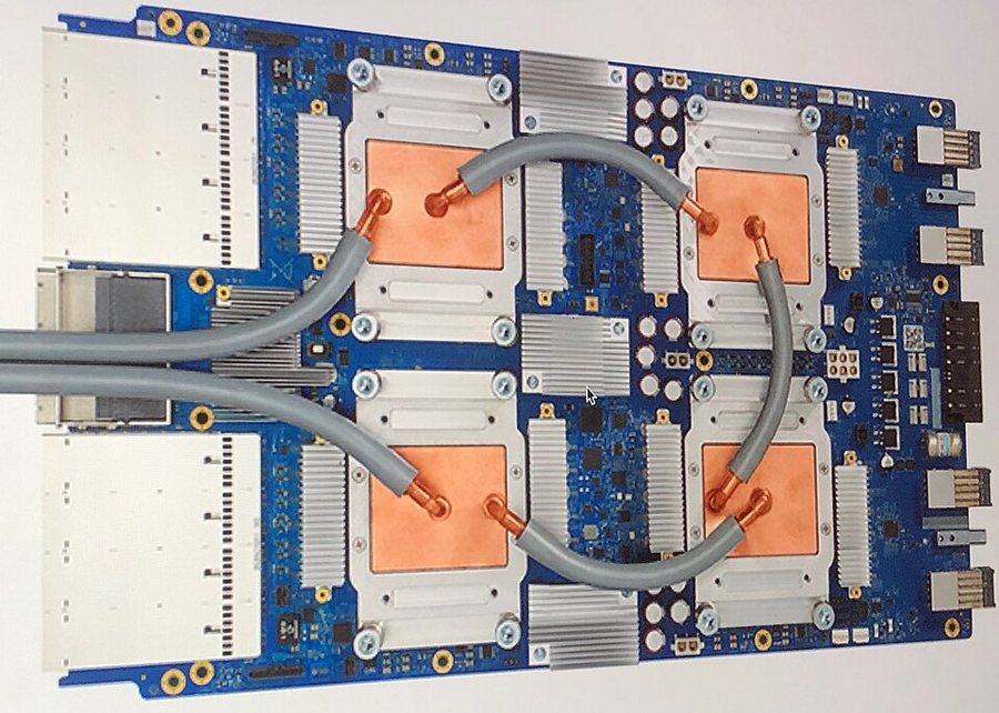
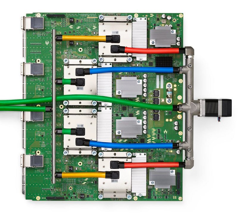
Google builds its own chips and joins them into **pods**. Gemini 1.5 was trained on several 4,096-chip pods of TPU v4, the report says. A TPU v5p chip does 459 trillion 16-bit FLOPs per second, and one pod holds 8,960 chips. Ironwood, announced in April 2025, puts 9,216 chips in a pod, with 4,614 trillion 8-bit FLOPs per second for each chip.
A TPU v3 board: four chips, each under a copper plate, cooled by liquid. Photo: Zinskauf, CC BY-SA 4.0, via Wikimedia Commons.A TPU v4 board, the chip generation that trained Gemini 1.5. Image: Norman P. Jouppi and colleagues, from their 2023 paper on TPU v4, CC BY 4.0, via Wikimedia Commons.
> [!DEFINITION] Model FLOPs utilisation (MFU)
> The share of the hardware's peak speed that goes into the model's useful arithmetic. Time spent waiting for data, talking between chips or recovering from failures lowers it.
No run reaches the peak. Llama 3 reports an MFU of 38% to 43% in 16-bit numbers. With those figures, our script estimates that $$3.8 \times 10^{25}$$ FLOPs on 16,384 H100s would take 63 to 71 days of pure training. That is our estimate, not a number Meta published.
### Splitting the work
A 405B model does not fit on one GPU, and one GPU would take centuries anyway. So the work is split in several ways at once.
> [!DEFINITION] Data, tensor and pipeline parallelism
> **Data parallelism** gives each GPU a full copy of the model and a different slice of each batch, then averages the gradients. **Tensor parallelism** splits each weight matrix across GPUs. **Pipeline parallelism** gives each GPU a block of consecutive layers, and passes activations along the chain.
With 4 stages and 4 micro-batches the pipeline is idle 3/7 of the time; with 32 micro-batches only 3/35 (8.6%). Numbers from our script.
Tensor parallelism comes from NVIDIA's Megatron-LM paper of 2019. It needs fast links, because GPUs must swap partial results inside every layer. So it usually stays within one server, where 8 GPUs are joined by NVLink.
> [!PAPER] Shoeybi et al. (2019), Megatron-LM: Training Multi-Billion Parameter Language Models Using Model Parallelism · Figure 3 · page 4
> [](/img/writings/history/h-megatron-fig.png)
>
> **What it says:** "Blocks of Transformer with Model Parallelism. f and g are conjugate. f is an identity operator in the forward pass and all reduce in the backward pass while g is an all reduce in the forward pass and identity in the backward pass."
>
> **What it means:**
>
> Split the first matrix by columns and the second by rows. Then each GPU can run its half of the feed-forward block with no talking in between. Only at the end, at $$g$$, do the two halves add up their results. Attention splits the same way, by heads. The paper trained an 8.3B model on 512 GPUs with 76% scaling efficiency, which was huge for 2019.
Take Llama 3 8B's feed-forward matrix of 4,096 × 14,336. Four GPUs would each hold a 4,096 × 3,584 slice; eight would each hold 4,096 × 1,792. Pipeline parallelism has a different cost: at the start and end of each batch, some stages sit idle while they wait. Cut the batch into $$m$$ **micro-batches** that flow through $$p$$ stages, and the idle share is
$$
\text{bubble} = \frac{p - 1}{m + p - 1}
$$
With 4 stages and 4 micro-batches, $$3/7 = 0.429$$ of the time is wasted. With 32 micro-batches it falls to $$3/35 = 0.086$$. With 16 stages and 64 micro-batches it is 0.190. More micro-batches shrink the bubble but need more memory. MoE models add a fourth kind, **expert parallelism**: different experts on different GPUs, with tokens sent to wherever their experts live. DeepSeek-V3 spread each layer's routed experts over 64 GPUs.
The [inference series](https://ishwarj.com/writings/llm-inference-7-beyond-one-gpu/) shows the same splits used for serving.
### Memory: sharding the optimizer
Training needs far more memory than the weights alone. In mixed-precision training with the Adam optimizer, each parameter needs 2 bytes for its 16-bit weight, and 2 for its 16-bit gradient. It also needs 12 bytes of 32-bit optimizer state: a master copy of the weight and Adam's two running averages. That is 16 bytes per parameter.
> [!DEFINITION] ZeRO and FSDP
> Methods that shard the optimizer states, gradients and even the weights across the GPUs of a data-parallel group, instead of copying them to every GPU. Each GPU keeps only its share and fetches the rest when needed. ZeRO is Microsoft's name; FSDP (fully sharded data parallel) is PyTorch's version.
For a 70B model, 16 bytes per parameter is 1,120 GB: the full memory of 14 GPUs with 80 GB each, before any activations. For 405B it is 6,480 GB. The ZeRO paper of 2019, from Samyam Rajbhandari and colleagues at Microsoft, gave the fix. Its example is a 7.5B model, which needs 120 GB of states. Sharded over 64 GPUs, each holds only 1.875 GB.
### Fewer bits per number
> [!DEFINITION] Mixed precision, bf16 and FP8
> Doing most arithmetic in short number formats while keeping a master copy of the weights in 32-bit. The **bf16** (brain floating point) format has 16 bits, with the range of 32-bit numbers but less precision. **FP8** uses only 8 bits, and needs careful scaling to avoid overflow.
Halving the bits halves the memory traffic and roughly doubles the speed of the matrix units. In 2017, Paulius Micikevicius and colleagues at NVIDIA and Baidu showed that 16-bit training works. You keep a 32-bit master copy and scale the loss. The bf16 format, with its wide range, made the scaling unnecessary and became the default.
DeepSeek-V3 was the first very large open model trained mostly in FP8. Its report says it was the first to "validate its effectiveness on an extremely large-scale model". The trick is to scale small blocks of numbers separately, so one large value does not ruin the precision of its neighbours. The most sensitive parts, such as the embedding, the output head and the normalisation, stay in higher precision.
### The optimizer and the schedule
Almost every large model is trained with **AdamW**, from Ilya Loshchilov and Frank Hutter (2017). It is like a hiker who keeps a running average of the slope and of how bumpy the slope has been. Steps are large where the ground is steady and small where it is noisy.
> [!DEFINITION] Learning rate
> The size of each training step: how far the weights move in the direction the gradient suggests. Too large and training becomes unstable; too small and it is slow.
$$
m_t = \beta_1 m_{t-1} + (1 - \beta_1) g_t, \quad v_t = \beta_2 v_{t-1} + (1 - \beta_2) g_t^2, \quad w_t = w_{t-1} - \eta \left( \frac{\hat m_t}{\sqrt{\hat v_t} + \epsilon} + \lambda w_{t-1} \right)
$$
$$g_t$$ is the gradient at step $$t$$. $$m_t$$ is the running average of gradients and $$v_t$$ of squared gradients, with decay rates $$\beta_1$$ and $$\beta_2$$. $$\hat m_t$$ and $$\hat v_t$$ are the same averages, corrected for starting at zero: divide by $$1 - \beta_1^t$$ and $$1 - \beta_2^t$$. $$\eta$$ (eta) is the learning rate and $$\lambda$$ (lambda) the **weight decay**, which pulls every weight a little toward 0.
Take one weight $$w = 1.0$$ with gradient $$g = 0.5$$, $$\eta = 0.001$$, $$\beta_1 = 0.9$$, $$\beta_2 = 0.95$$ and $$\lambda = 0.1$$. Then $$m = 0.05$$, $$v = 0.0125$$, $$\hat m = 0.5$$ and $$\hat v = 0.25$$. The Adam step is $$0.001 \times 0.5 / 0.5 = 0.001$$, the decay adds 0.0001, and the new weight is 0.9989. With $$g = 50$$, the step is still 0.001. Adam's first step has the size of the learning rate whatever the gradient's size, which is part of why it is stable.
DeepSeek-V3 used $$\beta_1 = 0.9$$, $$\beta_2 = 0.95$$ and weight decay 0.1, the same values as our example. The learning rate also changes during training. It starts at zero, rises in a straight line during a **warm-up**, and then falls.
$$
\eta(t) = \eta_{\min} + \tfrac{1}{2} (\eta_{\max} - \eta_{\min}) \left( 1 + \cos \frac{\pi (t - t_w)}{T - t_w} \right) \quad \text{for } t \ge t_w
$$
$$t$$ is the step, $$t_w$$ the length of the warm-up and $$T$$ the last step. $$\eta_{\max}$$ is the peak rate and $$\eta_{\min}$$ the final one. The cosine falls from 1 to $$-1$$, so the rate glides from the peak to the floor, slowly at first, then faster, then slowly again.
Llama 3 405B used a peak of $$8 \times 10^{-5}$$, 8,000 warm-up steps, and a cosine to $$8 \times 10^{-7}$$ over 1,200,000 steps. Our script assumes that the 1.2 million steps include the warm-up. Then the rate is $$4 \times 10^{-5}$$ at step 4,000 and $$4.04 \times 10^{-5}$$ half-way through, at step 604,000.
The warm-up is too short to see at this scale: 8,000 of 1,200,000 steps. Llama 3 then annealed the rate to 0 over the last 40 million tokens. Curve from our script.
Other shapes are common. DeepSeek-V3 held its peak rate flat until 10 trillion tokens and decayed it along a cosine over the next 4.3 trillion. It ended with two short flat steps. Chinchilla's lesson about schedules still holds: the decay must match the planned length of the run.
### When training breaks
> [!DEFINITION] Loss spike
> A sudden jump in the training loss, sometimes followed by recovery, sometimes by **divergence**, where the loss never comes back. Spikes become more common as models grow, and their causes are often unclear.
Large runs are fragile. Google's PaLM paper of 2022 is unusually frank about it. For its 540B model, the team "observed spikes in the loss roughly 20 times during training", although gradient clipping was on. Their fix was to restart "from a checkpoint roughly 100 steps before the spike started" and skip "roughly 200–500 data batches". The same batches, given to an earlier checkpoint, caused no spike. So the cause was the data and the model's state together, not bad data alone.
Since then, labs have added tricks such as extra normalisation inside attention and limits on the size of attention scores. DeepSeek-V3 reports that "we did not experience any irrecoverable loss spikes or perform any rollbacks". Kimi K2 used a new optimizer, MuonClip, and reports pre-training on 15.5 trillion tokens "with zero loss spike".
Hardware fails too. In one 54-day stretch of Llama 3 training, there were 466 interruptions. Of these, 419 were unexpected, and about 78% of those were traced to confirmed or suspected hardware problems. Google's Gemini 2.5 report describes the same problem at TPU scale.
> [!PAPER] Gemini Team, Google (2025), Gemini 2.5 · §2.3 · page 4
> [](/img/writings/history/h-gemini25-tpu.png)
>
> **What it says:** Gemini 2.5 is "the first to be trained on TPUv5p architecture", with "synchronous data-parallel training" over "multiple 8960-chip pods of Google's TPUv5p accelerators, distributed across multiple datacenters". "At the scale of this training run we see interruptions from hardware failures multiple times per hour."
>
> **What it means:**
>
> Several pods, in several buildings, act as one machine, and something breaks several times an hour. Google's answer is to keep going with fewer chips while a failed group is swapped out, at about 97% speed. The report adds that 93.4% of the run's time went into TPU work. At this scale, the engineering of failure is as important as the design of the model.
### What it costs
The most quoted cost in recent years comes from DeepSeek-V3, and it is often quoted wrongly.
> [!PAPER] DeepSeek-AI (2024), DeepSeek-V3 Technical Report · Table 1 and §1 · page 5
> [](/img/writings/history/h-dsv3-cost.png)
>
> **What it says:** pre-training took 2,664K H800 GPU hours, context extension 119K and post-training 5K, for 2,788K in total, or "$5.576M" at "$2 per GPU hour". Each trillion tokens took "180K H800 GPU hours, i.e., 3.7 days on our cluster with 2048 H800 GPUs". The costs cover "only the official training", "excluding the costs associated with prior research and ablation experiments".
>
> **What it means:**
>
> The table is the rent for the final run, at an assumed price. It is not the cost of the company, its chips, its staff or the many smaller runs that found the recipe. The numbers check out: 180K hours times 14.8 trillion tokens is 2,664K. Spread over 2,048 GPUs, 2,664K hours is about 54 days. It was still a striking result for a model of its quality.
Our script adds one more check. With $$C = 6 \times 37 \times 10^9 \times 14.8 \times 10^{12} = 3.29 \times 10^{24}$$ FLOPs over 2,664K GPU hours, each GPU did about 343 trillion useful FLOPs per second. That leaves out attention, and it is our estimate, not DeepSeek's. Closed labs do not publish their training costs at all.
### Predicting more than one token
DeepSeek-V3 also trained with **multi-token prediction**. Besides the next token, a small extra module predicts the token after it.
> [!DEFINITION] Multi-token prediction (MTP)
> A training objective where the model predicts several future tokens at each position, not only the next one. It gives more training signal per token, and the extra predictions can later speed up generation.
Fabian Gloeckle and colleagues at Meta studied the idea in 2024. Their models trained with 4-token prediction were "up to 3× faster at inference". DeepSeek-V3 used a depth of 1, one extra token. It reports that the extra prediction is accepted 85% to 90% of the time, which gives about 1.8 times more tokens per second. The next section shows where that number comes from.
## Built for serving
A model is trained once and served for months to millions of people, so its design is shaped by serving costs. GQA, MLA and MoE are all, in part, serving decisions. Three more tricks matter.
### Speculative decoding
> [!DEFINITION] Speculative decoding
> A way to generate faster with no change to the output. A small, fast **draft** model guesses several tokens. The large model checks them all in one pass. It keeps the guesses that match its own choices and fixes the first wrong one.
Writing one token at a time leaves a GPU mostly idle, because each step reads all the weights to make one token. Checking five guessed tokens costs about the same as making one. In 2022, Yaniv Leviathan and colleagues at Google showed a 2X-3X speed-up on T5-XXL "with identical outputs". If each guess is accepted with probability $$a$$ and the draft guesses $$\gamma$$ tokens, each pass of the large model yields on average
$$
\mathbb{E}[\text{tokens per pass}] = \frac{1 - a^{\gamma + 1}}{1 - a}
$$
$$a$$ is the acceptance rate and $$\gamma$$ (gamma) is the draft length. The formula counts the accepted guesses plus the one token the large model always adds. With $$a = 0.8$$ and $$\gamma = 4$$, that is 3.362 tokens per pass; with $$a = 0.6$$, 2.306.
DeepSeek-V3 uses its MTP module as the draft, with $$\gamma = 1$$. At $$a = 0.85$$ the formula gives 1.850 tokens per pass, and at 0.9 it gives 1.900. That agrees with the 1.8 times speed-up the report gives. The [inference series](https://ishwarj.com/writings/llm-inference-4-speculative-decoding/) covers the method in depth.
### Quantisation
Part 1 introduced **quantisation**: storing weights in fewer bits. A 70B model needs 140 GB at 16 bits, 70 GB at 8 bits and 35 GB at 4 bits. DeepSeek-V3's 671B parameters take about 671 GB in FP8, the format it was trained in. Many open models are now released in 8-bit or 4-bit versions, and serving systems run them with special matrix kernels.
### Distillation into small models
Most users talk to small models. Labs make them by **distillation**, defined in [Part 4](https://ishwarj.com/writings/how-models-are-trained-today/): a small student learns from a big teacher's outputs. In pre-training, the student learns from the teacher's full probability over the next token, not only from the one token in the text. That is a far richer signal: it says that "cat" was likely, "dog" was nearly as likely, and "car" was not.
> [!PAPER] Gemini Team, Google (2025), Gemini 2.5 · §2.1 · page 3
> [](/img/writings/history/h-gemini25-distill.png)
>
> **What it says:** the smaller Gemini 2.5 models, Flash size and below, "use distillation", "as was done in the Gemini 1.5 series". To save storage, the teacher's next-token distribution is approximated "using a k-sparse distribution over the vocabulary".
>
> **What it means:**
>
> "k-sparse" means that only the teacher's top $$k$$ tokens and their probabilities are stored for each position, not all of the vocabulary. Even so, the data grows by a factor of $$k$$, and Google says the quality gain is worth it. The Gemini 1.5 report says that 1.5 Flash was "online distilled" from 1.5 Pro, meaning it learned while the teacher ran alongside it.
Google's open Gemma models follow the same path: the Gemma 3 report says that "all Gemma 3 models are trained with knowledge distillation". Meta used the 405B model to improve its smaller Llama 3 models in post-training, and Qwen3 describes "strong-to-weak distillation". The big model's main job in a family is often to teach the small ones.
## What labs publish, and what they do not
Everything in this part comes from papers, technical reports and model cards. They differ widely in how much they say.
> [!DEFINITION] Model card and technical report
> A **model card** is a short document that a lab publishes with a model. It says what the model is for, how it was evaluated, and its limits and safety tests. A **technical report** is longer and may describe the architecture, data and training, but labs choose what to put in it.
The open-weight labs publish the most: DeepSeek, Meta's Llama papers, Qwen, Kimi and above all the Allen Institute's Olmo, which also releases its data. Google's Gemini reports confirm the design in outline: sparse MoE, natively multimodal, long context, TPUs, distillation for the small models. OpenAI's GPT-4 report of 2023 set the closed pattern. It "contains no further details about the architecture (including model size), hardware, training compute, dataset construction, training method, or similar."
| Question | Open-weight reports (DeepSeek, Llama, Olmo) | Closed frontier labs |
|---|---|---|
| Layer design | Full: norms, attention type, sizes | Google: "sparse MoE", little more; others: nothing |
| Parameter count | Exact, total and active | Not published |
| Training tokens | Exact or close | Not published |
| Data sources | Described; Olmo releases the data | Categories only ("web documents, code, images") |
| Hardware | Chip type and count | Google names TPU generations; others: little |
| Cost | DeepSeek: GPU hours for the final run | Not published |
So, when you read a claim about a closed model's size or cost, ask where it comes from. If it is not in a lab's own report or model card, it is a guess or a leak, however often it is repeated.
## How the five parts fit together
Put the parts of this series side by side and you get the whole build of a frontier model in 2026.
A composite of the Llama 3, DeepSeek-V3, Gemini 2.5 and Olmo 3 reports. Closed labs confirm only parts of it.
[Part 1](https://ishwarj.com/writings/from-neuron-to-opus/) gave the parts list: the neuron, backpropagation, attention, the Transformer, the next-token loss. This part showed what they look like at scale. Part 2's classical methods live on inside the pipeline, as the small fast classifiers that filter data. [Part 3](https://ishwarj.com/writings/reinforcement-learning-history/) and [Part 4](https://ishwarj.com/writings/how-models-are-trained-today/) take over once the base model exists, and turn it into an assistant that reasons and uses tools.
The lessons repeat across all five parts. A good loss is not the same as a good model. Goodhart's law in Part 4 and the warning about loss in this part both show it. Scale wins, but only when the bottleneck moves: from compute to data, from data to memory, from memory to the cost of every answer. And most progress is a chain of fixes, each solving the limit the step before it left behind.
## What is still open
Data is the hardest limit. Good public text is close to used up, so the future depends on synthetic data, other kinds of data and better reuse. Whether a model can learn as much from text written by models as from text written by people is still an open question.
Architecture is less settled than it looks. Many 2025 and 2026 models mix in other layer types, such as linear attention, state-space layers and sparse attention, to make long contexts cheaper. The [attention series](https://ishwarj.com/writings/attention-4-linear-hybrid/) covers them. DeepSeek-V3.2 added its own sparse attention. The SwiGLU paper's "divine benevolence" is still a fair summary of how many of these choices are made.
And scaling itself is changing shape. Pre-training compute keeps growing, but more of the total now goes to post-training and to thinking at answer time, as Part 4 showed. The next part of the curve may be drawn on that second axis.
| Step | What it fixed | What it left open |
|---|---|---|
| Next-token loss, perplexity | One clear goal for raw text | Loss is not ability |
| Kaplan scaling laws (2020) | Predictable gains from small runs | Wrong split between size and data |
| Chinchilla (2022) | Compute-optimal size and data | Ignores the cost of serving |
| Over-training (Llama 3, 2024) | Small models that are cheap to serve | Needs ever more data |
| Filtering, dedup, quality classifiers | Better data from the same web | Hard to test; can tilt the data |
| Byte-level BPE | Any text in a fixed vocabulary | Uneven cost across languages |
| Pre-norm, RMSNorm, SwiGLU | Stable, cheaper deep stacks | Found by trial, not theory |
| RoPE and its scaling | Relative positions; longer contexts | Quality falls far past the training length |
| FlashAttention | Exact attention without the $$n^2$$ memory | Still $$n^2$$ arithmetic |
| MQA, GQA, MLA | A much smaller KV cache | Extra design and tuning |
| Mixture of experts | More knowledge per FLOP | Load balance, memory, communication |
| Parallelism, ZeRO, FP8 | Training across thousands of chips | Failures, loss spikes, cost |
| Speculative decoding, quantisation, distillation | Cheaper, faster serving | Small models trail the big ones |
> [!TAKEAWAYS]
> - Pre-training minimises one number, the next-token cross-entropy; perplexity is its exponential.
> - Training compute is about $$6ND$$. Kaplan showed smooth power laws; Chinchilla showed that size and data should grow together, near 20 tokens per parameter.
> - Labs now over-train small models on far more tokens than that, because a smaller model is cheaper for every user. The limit is now the supply of good data.
> - Pre-training data is the filtered web: extraction, language checks, rules, deduplication and quality classifiers. It is mixed with code, maths, other languages and synthetic text, and ends with an annealing phase.
> - The 2026 decoder layer keeps the Transformer's skeleton but uses pre-norm RMSNorm, SwiGLU, RoPE and shared keys and values (GQA or MLA); FlashAttention makes attention fit the memory of the chip.
> - Mixture-of-experts layers send each token to a few experts chosen by a router, so total size and cost per token come apart; DeepSeek-V3 uses 37B of 671B parameters per token, and Gemini is a sparse MoE.
> - Training spreads one model over thousands of GPUs or TPUs with data, tensor, pipeline and expert parallelism. It shards the optimizer states, uses 16-bit or 8-bit numbers, and must survive constant hardware failures.
> - Open-weight labs publish their designs in detail; closed labs publish outlines, so claims about closed models need a source.
Key papers: [Kaplan et al. 2020](https://arxiv.org/abs/2001.08361), [Chinchilla 2022](https://arxiv.org/abs/2203.15556), [Llama 3 2024](https://arxiv.org/abs/2407.21783). Data and architecture: [FineWeb 2024](https://arxiv.org/abs/2406.17557), [BPE 2016](https://arxiv.org/abs/1508.07909), [RoFormer 2021](https://arxiv.org/abs/2104.09864), [FlashAttention 2022](https://arxiv.org/abs/2205.14135). Experts and scale: [Switch Transformer 2021](https://arxiv.org/abs/2101.03961), [DeepSeek-V3 2024](https://arxiv.org/abs/2412.19437), [Gemini 2.5 2025](https://arxiv.org/abs/2507.06261).
Back to [Part 4, From RLHF to Reasoning](https://ishwarj.com/writings/how-models-are-trained-today/), or to the start of the series, [Part 1, From One Neuron to Opus](https://ishwarj.com/writings/from-neuron-to-opus/).