# Classical Machine Learning: From Least Squares to XGBoost
Author: Ishwar Jangid
Canonical URL: https://ishwarj.com/writings/classical-machine-learning/
Updated: 2026-10-22
Source: https://github.com/ishwar6/ishwar-books/blob/main/content/writings/classical-machine-learning.md
A bank must decide whether to approve a loan. It has a table: one row per past customer, with columns for income, debt, age of the account and whether the loan was repaid. A spam filter has a similar job with words instead of columns. Neither needs a model with billions of parameters. For problems like these, a family of older methods is often faster, cheaper and just as accurate.
[Part 1](https://ishwarj.com/writings/from-neuron-to-opus/) followed neural networks from the 1943 neuron to today's Claude models. This part follows the other branch: the statistical methods that learn from examples without deep networks. Some of them are more than two hundred years old. During the 1990s and 2000s, while neural networks were out of fashion, these methods were machine learning. Each section gives the key equation, with small numbers you can check by hand. [Part 3](https://ishwarj.com/writings/reinforcement-learning-history/) covers reinforcement learning, [Part 4](https://ishwarj.com/writings/how-models-are-trained-today/) covers how language models are trained today, and [Part 5](https://ishwarj.com/writings/inside-a-modern-language-model/) covers how the base model is built.
> [!TIP] The whole idea in one minute
> Every method here answers the same question: given examples with known answers, how do you predict the answer for a new one?
>
> **Regression** fits a line. **Nearest neighbours** copies the answer of the most similar past example. **Naive Bayes** counts evidence. **Decision trees** ask a short list of yes-or-no questions. **Support vector machines** draw the widest possible border. **Ensembles** combine many weak models into a strong one, and gradient boosting, as in XGBoost, is the strongest of these on tables of data.
## 1805 to 1958: fitting lines to data
### Least-squares regression
Learning from examples is much older than AI. Around 1805, Adrien-Marie Legendre published the **method of least squares**, and Carl Friedrich Gauss published his version in 1809. They used it to fit the orbits of planets and comets to noisy measurements. It is still the first model most people learn.
Imagine pushing a stiff ruler through a cloud of dots, where each dot is tied to the ruler by a small spring. The ruler settles where the total stretch of the springs is smallest. Least squares finds that position.
> [!DEFINITION] Linear regression
> A model that predicts a number as a weighted sum of inputs plus a constant, for example a house price from its size. Fitting it means choosing the weights that make the predictions closest to the known answers.
$$
\min_{w,\,b} \; \sum_{i=1}^{n} \big( y_i - (w x_i + b) \big)^2
$$
Here $$n$$ is the number of examples, $$x_i$$ is the input of example $$i$$ and $$y_i$$ is its true answer. The term $$w x_i + b$$ is the prediction of a straight line with slope $$w$$ and intercept $$b$$. The difference $$y_i - (w x_i + b)$$ is the error of that prediction. Squaring the error makes it positive and punishes big errors more than small ones. "min" means we choose the $$w$$ and $$b$$ that make the sum as small as possible.
Take three points: $$(1, 2)$$, $$(2, 4)$$ and $$(3, 5)$$. The best slope is the covariance of $$x$$ and $$y$$ divided by the variance of $$x$$.
The means are $$\bar{x} = 2$$ and $$\bar{y} = 11/3 \approx 3.67$$. The sum of $$(x_i - \bar{x})(y_i - \bar{y})$$ is $$1.67 + 0 + 1.33 = 3$$, and the sum of $$(x_i - \bar{x})^2$$ is 2. So $$w = 1.5$$ and $$b = 3.67 - 1.5 \times 2 \approx 0.67$$. The line predicts 2.17, 3.67 and 5.17, and the sum of squared errors is about 0.17. No other straight line does better on these three points.
> [!DEFINITION] Loss function
> A number that measures how wrong a model is on its data. The sum of squared errors above is one loss function. Training a model means making its loss small.
Least squares has a formula for the best line. Most models in this part do not. They are trained step by step with **gradient descent**, the "walk downhill in the fog" method that Part 1 explains.
### Galton names regression
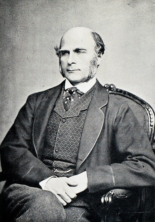
The word "regression" comes from the British scientist Francis Galton. In 1886, he compared the heights of parents and their adult children. Very tall parents tended to have children who were tall, but less extreme. He called this "regression towards mediocrity", a pull back toward the average. The line he fitted to show it gave the whole method its name.
Francis Galton in the 1850s. Public domain, via Wikimedia Commons.
### Logistic regression
Many questions have a yes-or-no answer: will this customer leave, is this email spam, will this loan be repaid? A straight line can give any number, such as 1.7 or $$-3$$, which is not a probability. In 1958, the statistician David Cox described **logistic regression**. It takes the same weighted sum and squeezes it into the range 0 to 1 with the **sigmoid** function.
It is like a dimmer switch. A weighted sum far below zero means "almost certainly no", far above zero means "almost certainly yes", and zero means "50-50".
$$
p = \sigma(z) = \frac{1}{1 + e^{-z}}, \qquad z = \sum_j w_j x_j + b
$$
$$z$$ is the weighted sum of the inputs $$x_j$$ with weights $$w_j$$, plus the bias $$b$$. $$e$$ is the number 2.718. $$\sigma(z)$$ is the sigmoid of $$z$$, and $$p$$ is the predicted probability of "yes". The model is trained with the **log loss**: $$-\ln p$$ when the true answer is yes, and $$-\ln(1 - p)$$ when it is no.
Take one input $$x = 1.5$$, with $$w = 2$$ and $$b = -1$$. Then $$z = 2 \times 1.5 - 1 = 2$$, and $$p = 1 / (1 + e^{-2}) = 1 / 1.135 \approx 0.88$$. If the true answer is yes, the log loss is $$-\ln 0.88 \approx 0.13$$, small. If the true answer is no, it is $$-\ln 0.12 \approx 2.1$$, large. Logistic regression is still a strong first choice for yes-or-no questions, and the same sigmoid sits inside early neural networks.
## 1951 to 1967: learning by looking at neighbours
### The nearest-neighbour rule
The simplest way to predict is to find the most similar past case and copy its answer. A doctor does this when they say "this looks like the case we saw last month". In 1951, Evelyn Fix and Joseph Hodges described this rule in a report for the US Air Force. In 1967, Thomas Cover and Peter Hart proved how good it can be. With enough data, its error is at most twice the best possible error.
> [!DEFINITION] k-nearest neighbours (k-NN)
> A method that predicts the answer for a new example from the $$k$$ training examples closest to it. Those examples vote with their answers.
Closeness needs a distance. The usual one is the straight-line distance:
$$
d(\mathbf{a}, \mathbf{b}) = \sqrt{\sum_{j} (a_j - b_j)^2}
$$
$$\mathbf{a}$$ and $$\mathbf{b}$$ are two examples, each a list of measurements. $$a_j$$ and $$b_j$$ are their values in measurement $$j$$. The sum adds up the squared differences in every measurement, and the square root turns the total back into a distance.
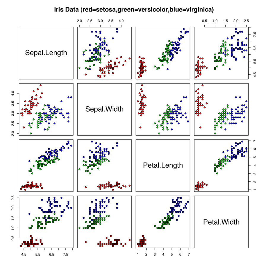
A famous test case is the iris flower data, which the statistician Ronald Fisher published in 1936. It has 150 flowers of three species, with four measurements each. Plot any two measurements against each other, and the species form clear clusters.
The iris data: every pair of the four measurements, coloured by species (red setosa, green versicolor, blue virginica). Plot by Indon, CC BY-SA 3.0, via Wikimedia Commons.
Now classify a new flower with petal length 1.5 cm and petal width 0.3 cm, against three stored flowers. Say flower A (1.4, 0.2) is a setosa, at distance $$\sqrt{0.01 + 0.01} \approx 0.14$$. Flower C (1.3, 0.4) is also a setosa, at distance $$\sqrt{0.04 + 0.01} \approx 0.22$$. Flower B (4.5, 1.5) is a versicolor, at distance $$\sqrt{9 + 1.44} \approx 3.23$$. With $$k = 3$$, the vote is two setosa against one versicolor, so the new flower is a setosa.
Nearest neighbours needs no training at all, only storage. Its cost is at prediction time: it must compare each new example with every stored one. The same idea, with smarter search structures, powers today's vector search, where a model's embeddings are compared to find similar documents.
## Counting evidence: Naive Bayes
### Bayes' rule
Some words make an email more likely to be spam: "free", "winner", "urgent". No single word is proof, but each one adds evidence. Bayes' rule, from an essay by Thomas Bayes published in 1763 after his death, says how to update a belief when new evidence arrives.
$$
P(A \mid B) = \frac{P(B \mid A)\, P(A)}{P(B)}
$$
$$P(A)$$ is the belief in $$A$$ before the evidence, for example "this email is spam". $$P(B \mid A)$$ is how likely the evidence $$B$$ is when $$A$$ is true, for example "spam emails contain *free*". $$P(B)$$ is how likely the evidence is overall. $$P(A \mid B)$$ is the updated belief after seeing the evidence.
### The naive step
**Naive Bayes** applies the rule to many pieces of evidence at once. It makes one bold, "naive" assumption: that each word appears independently of the others, once you know the class. The assumption is false (the words "free" and "offer" often come together), but the method works well anyway.
M. E. Maron used it to sort documents by subject in 1961. In 2002, the programmer Paul Graham's essay "A Plan for Spam" made Bayesian spam filters popular.
> [!DEFINITION] Naive Bayes
> A classifier that multiplies the probability of each class by the probability of each observed feature in that class. It treats the features as independent and picks the class with the largest result.
$$
P(\text{spam} \mid w_1, \dots, w_n) \propto P(\text{spam}) \prod_{i=1}^{n} P(w_i \mid \text{spam})
$$
$$w_1$$ to $$w_n$$ are the words in the email. $$P(w_i \mid \text{spam})$$ is the share of spam emails that contain word $$w_i$$. The symbol $$\prod$$ means "multiply all of them", and $$\propto$$ means "is proportional to". We compute the same product for "not spam" and compare the two.
Say 40% of emails are spam. "Free" appears in 50% of spam and 5% of normal email. "Meeting" appears in 10% of spam and 30% of normal email.
An email contains both words. The spam score is $$0.4 \times 0.5 \times 0.1 = 0.02$$. The normal score is $$0.6 \times 0.05 \times 0.3 = 0.009$$. So the chance of spam is $$0.02 / (0.02 + 0.009) \approx 0.69$$. The word "meeting" pulled it down, but "free" won.
## 1984: decision trees and CART
A decision tree is the game of twenty questions. To guess an animal, you ask "does it fly?", then "is it bigger than a cat?", and each answer cuts the options down. A tree model learns which questions to ask, and in what order, from the data.
In 1984, Leo Breiman, Jerome Friedman, Richard Olshen and Charles Stone published *Classification and Regression Trees*, known as **CART**. Ross Quinlan published the related ID3 algorithm in 1986 and C4.5 in 1993. CART grows a tree by trying every possible question at each node and keeping the one that makes the groups below it the most "pure".
> [!DEFINITION] Decision tree
> A model that predicts by asking a sequence of yes-or-no questions about the input, such as "is age above 40?". Each answer leads down a branch. The last node, a **leaf**, gives the prediction.
CART measures purity with the **Gini impurity**. It is the chance that two items drawn at random from a group, with replacement, belong to different classes.
$$
G = 1 - \sum_{k=1}^{K} p_k^2
$$
$$K$$ is the number of classes and $$p_k$$ is the share of items in the group that belong to class $$k$$. A group with only one class has $$G = 0$$. A group split evenly between two classes has $$G = 0.5$$, the worst case for two classes. To score a question, CART computes the Gini of each child group, weights each by its share of the items, and adds them.
Take ten emails: five spam and five not.
The Gini at the top is $$1 - (0.5^2 + 0.5^2) = 0.5$$. Try the question "does it contain the word *free*?". Four emails say yes, and all four are spam, so that group has $$G = 0$$. Six say no: one spam and five not, so $$G = 1 - (1/36 + 25/36) \approx 0.28$$. The weighted score is $$0.4 \times 0 + 0.6 \times 0.28 \approx 0.17$$. The question lowers the impurity from 0.5 to 0.17, so it is a good split.
> [!DEFINITION] Overfitting
> When a model learns the noise and quirks of its training examples instead of the real pattern. It then scores well on the examples it saw and badly on new ones.
Trees are easy to read and need little data preparation. Their weakness is that one deep tree overfits. It memorises the training examples, and a small change in the data can give a very different tree. The ensembles below fix exactly this.
## 1992 to 1995: support vector machines
### The widest street
In the 1990s, the strongest general-purpose classifier was the **support vector machine**. Bernhard Boser, Isabelle Guyon and Vladimir Vapnik described its nonlinear form in 1992, and Corinna Cortes and Vapnik published the "soft margin" version in 1995.
Picture two groups of coins on a table. Many lines can separate them. The SVM picks the line that leaves the widest empty street between the two groups. A wide street makes the model less sensitive to small changes in new data.
> [!DEFINITION] Support vector machine (SVM)
> A classifier that separates two classes with the line or plane that has the largest margin, the widest gap to the nearest examples. Those nearest examples are the **support vectors**.
$$
\min_{\mathbf{w},\, b} \; \tfrac{1}{2} \lVert \mathbf{w} \rVert^2 \quad \text{subject to} \quad y_i \,(\mathbf{w} \cdot \mathbf{x}_i + b) \ge 1 \text{ for every } i
$$
The border is the set of points where $$\mathbf{w} \cdot \mathbf{x} + b = 0$$. Each example $$\mathbf{x}_i$$ has a label $$y_i$$ of $$+1$$ or $$-1$$. The condition says every example must sit on its own side, at least one unit past the border. The width of the street is $$2 / \lVert \mathbf{w} \rVert$$, so making $$\lVert \mathbf{w} \rVert$$ small makes the street wide.
Say the best border has $$\lVert \mathbf{w} \rVert = 2$$. Then the street is $$2 / 2 = 1$$ unit wide. A border with $$\lVert \mathbf{w} \rVert = 1$$ that still keeps every point on its side would give a street 2 units wide, and the SVM would prefer it. The "soft margin" version of 1995 lets a few points sit inside the street, at a price. One odd example then cannot ruin the border.
### The kernel trick
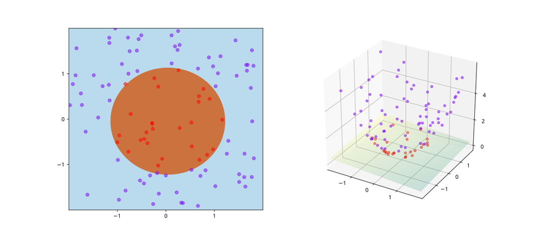
Some classes cannot be split by a straight line at all, such as a ring of points around a central cluster. The kernel trick lifts the data into more dimensions, where a flat plane can split it.
> [!DEFINITION] Kernel trick
> A way to let an SVM draw curved boundaries. It compares examples with a **kernel**, a similarity function. The kernel acts like a dot product in a much larger feature space, without ever computing that space.
The kernel trick. On the left, no straight line separates the inner points from the outer ring. Lifted into three dimensions on the right, a flat plane does. Image by Shiyu Ji, CC BY-SA 4.0, via Wikimedia Commons.
SVMs had clean math and strong guarantees, and they beat neural networks on many tasks of the time. Their cost grows fast with the number of training examples, and they still needed people to design good input features by hand. Both limits mattered later, when data sets reached millions of images.
## 1995 to 2001: many weak voices, one strong answer
### Ensembles
In 1906, Francis Galton looked at a contest at a country fair where about 800 people guessed the weight of an ox. Each guess was noisy, but the middle of all guesses was close to the true weight. Ensembles use the same effect. Many models that are each a bit wrong, in different ways, can be combined into one model that is more often right.
> [!DEFINITION] Ensemble
> A model that combines the predictions of many smaller models, for example by voting or by adding them up.
There are two main ways to build one. **Bagging** trains many models in parallel on different random samples of the data and averages them. **Boosting** trains models one after another, and each new model focuses on the mistakes of the ones before it.
### AdaBoost and random forests
Yoav Freund and Robert Schapire introduced **AdaBoost** in 1995, with the journal version in 1997. It gives more weight to the training examples that earlier models got wrong. Each new model works hardest on the cases the team still misses.
Leo Breiman published **random forests** in 2001. A random forest grows hundreds of deep trees and lets them vote. Each tree sees a random sample of rows, and a random subset of columns at each split. The randomness makes the trees disagree, and the vote cancels much of their overfitting.
> [!PAPER] Breiman (2001), Random Forests · Abstract · page 1
> [](/img/writings/history/h-rf.png)
>
> **What it says:** random forests are "a combination of tree predictors" where each tree depends on an independent random vector. With "a random selection of features to split each node", the error rates "compare favorably to Adaboost". The forests are also more robust to noise.
>
> **What it means:**
>
> The abstract names the two forces that decide how good a forest is: the strength of each tree and the correlation between them. Strong trees help, but trees that all make the same mistake do not. Choosing a random subset of columns at each split forces the trees to differ. A forest of different, fairly good trees beats one excellent tree.
## 2001 to 2017: gradient boosting and XGBoost
### Gradient boosting
Also in 2001, Jerome Friedman published "Greedy function approximation: a gradient boosting machine". He saw boosting as gradient descent, but in the space of functions instead of weights. Each new tree is a step downhill.
Think of a golfer. The first shot lands short of the hole. The second shot does not start again from the tee: it aims at the remaining distance. Each shot corrects what is left. Gradient boosting builds its prediction the same way:
$$
F_m(x) = F_{m-1}(x) + \nu \, h_m(x)
$$
$$F_{m-1}(x)$$ is the prediction after $$m - 1$$ trees. $$h_m(x)$$ is a new small tree, trained to predict the current errors. For squared loss, those errors are the **residuals** $$r_i = y_i - F_{m-1}(x_i)$$, which are also the negative gradient of the loss. The **shrinkage** factor $$\nu$$ (nu), often 0.1 or smaller, makes each step small so that no single tree has too much say.
Say a house sells for 300 (in thousands). The first guess $$F_0$$ is the average price, 250, so the residual is 50. The first tree predicts a residual of 40 for this house. With $$\nu = 0.1$$, the new prediction is $$250 + 0.1 \times 40 = 254$$. The residual is now 46, and the next tree aims at that. After hundreds of trees, the small steps add up to an accurate prediction.
### XGBoost
In 2016, Tianqi Chen and Carlos Guestrin published **XGBoost** at the KDD conference. It is gradient boosting with careful engineering. It uses second derivatives for better steps and adds a penalty on tree size and leaf values. It also handles missing values and runs in parallel.
> [!PAPER] Chen and Guestrin (2016), XGBoost: A Scalable Tree Boosting System · Abstract · page 1
> [](/img/writings/history/h-xgb-abs.png)
>
> **What it says:** the paper describes "a scalable end-to-end tree boosting system called XGBoost". With new algorithms for sparse data and careful use of memory, it "scales beyond billions of examples" with far fewer resources than earlier systems.
>
> **What it means:**
>
> The math of gradient boosting was fifteen years old. What XGBoost added was speed and scale: it made boosting practical on very large tables and on ordinary hardware. That is why it spread so fast.
XGBoost adds a penalty to the loss so that the trees stay simple:
$$
\mathcal{L} = \sum_{i} l(y_i, \hat{y}_i) + \sum_{k} \Big( \gamma T_k + \tfrac{1}{2} \lambda \lVert w_k \rVert^2 \Big)
$$
The first sum is the usual loss $$l$$ between each true answer $$y_i$$ and the prediction $$\hat{y}_i$$. The second sum runs over the trees $$k$$. $$T_k$$ is the number of leaves of tree $$k$$, and $$w_k$$ are the values in its leaves. $$\gamma$$ (gamma) charges a price for every extra leaf, and $$\lambda$$ (lambda) charges a price for large leaf values.
Take one possible split. Say it would lower the loss by 0.8 but add one leaf, and $$\gamma = 1$$. The total change is $$-0.8 + 1 = +0.2$$, so the loss goes up and XGBoost does not make the split. With $$\gamma = 0.5$$, the change is $$-0.3$$ and the split is kept. A larger $$\gamma$$ gives smaller, simpler trees.
> [!PAPER] Chen and Guestrin (2016), XGBoost: A Scalable Tree Boosting System · §1 · page 1
> [](/img/writings/history/h-xgb-kaggle.png)
>
> **What it says:** "Among the 29 challenge winning solutions" published on the blog of the competition site Kaggle during 2015, "17 solutions used XGBoost".
>
> **What it means:**
>
> Kaggle competitions are a hard public test: thousands of teams try every method on the same data. More than half of the winning solutions that year used one library. LightGBM from Microsoft and CatBoost from Yandex followed in 2017 with the same core idea and different speed tricks.
## Why trees still win on tables
> [!DEFINITION] Tabular data
> Data in a table, where each row is one item (a customer, a loan, a house) and each column is one property. Spreadsheets and SQL databases hold tabular data.
Deep learning took over images, sound and text in the 2010s. Those kinds of data have a shape: pixels next to pixels, words after words. Convolutions and attention use that shape. A table has no such shape. Column 3 (income) has no special relation to column 4 (postcode), and the order of the columns means nothing.
> [!PAPER] Grinsztajn, Oyallon and Varoquaux (2022), Why do tree-based models still outperform deep learning on typical tabular data? · Abstract · page 1
> [](/img/writings/history/h-tabular.png)
>
> **What it says:** the paper tests a standard set of "45 datasets" with clear tabular features. "Tree-based models remain state-of-the-art on medium-sized data" of about 10,000 samples, even before counting their speed.
>
> **What it means:**
>
> This was a careful test, with a large search for good settings for every model. Trees still won on the typical business table. The paper's explanation is that trees cope well with useless columns and with sharp, irregular patterns. An example is a rule that changes at an exact age or price.
So the two branches of this series solve different problems. For a table of a few thousand to a few million rows, a team usually starts with gradient-boosted trees. They train in minutes, need little tuning and are easy to explain. For images, sound, text and code, deep networks win, and large language models now handle many tasks with no task-specific training at all. Many real systems use both: a language model reads the documents, and a boosted tree makes the final score.
> [!TAKEAWAYS]
> - Learning from examples began with least squares around 1805, long before computers. Galton's 1886 study gave regression its name.
> - Logistic regression turns a weighted sum into a probability with the sigmoid, and it remains a strong first model for yes-or-no questions.
> - Nearest neighbours copies the answer of the most similar past examples; Naive Bayes multiplies the evidence of each feature.
> - Decision trees choose their questions by how much they lower the Gini impurity, but one deep tree overfits.
> - Support vector machines draw the widest possible border, and the kernel trick lets them draw curved ones.
> - Ensembles fix overfitting: random forests average many different trees, and boosting adds small trees that correct the remaining errors.
> - XGBoost made gradient boosting fast at scale, and on typical tables of data, boosted trees still beat deep learning.
Key papers: [Breiman, Random Forests (2001)](https://www.stat.berkeley.edu/~breiman/randomforest2001.pdf), [Chen and Guestrin, XGBoost (2016)](https://arxiv.org/abs/1603.02754), [Grinsztajn et al. (2022)](https://arxiv.org/abs/2207.08815).
Back to [Part 1, From One Neuron to Opus](https://ishwarj.com/writings/from-neuron-to-opus/), the neural network line from 1943 to today.